
GoodFitSBM (Version 0.0.1): GoodFitSBM comprises functionality that performs the goodness-of-fit test for an ER-SBM as well as a beta-SBM (two of the three variants of SBMs as discussed in Karwa et al. (2023), used for modelling network data).
The math rendering of README.md is not ideal, as a result of which most of the math notations and equations remains un-rendered, hence knit the README.Rmd, or refer to the PDF attached as README.pdf.
Stochastic blockmodels (SBMs) contributed to the theoretical and algorithmic developments for analyzing network data, which has been facilitated by the availability of data in diverse fields like social sciences, web recommender systems, protein networks, genomics, and neuroscience. SBMs being the generalization of the Erdős-Rényi model given by Erdős and Rényi (1960) was proposed originally in context of social sciences for directed and undirected graphs, whereas now it has been vastly extended and utilized in latent blocks in undirected graphs, latent space models, variable degree distribution, dynamically evolving networks, etc., becoming one of the more popular approaches to model network data in computer science, statistics and machine learning.
Karwa et al. (2023) addresses a very important aspect of model fitting by constructing (exact) goodness-of-fit tests (under finite-sample setting) for three variants of SBMs respectively used for modeling network data (where model adequacy procedures are somewhat elusive in general), viz., Erdős-Rényi SBM (ER-SBM), Additive SBM, and beta-SBM, where the main idea revolves around a frequentist conditional goodness-of-fit test conditioned on a sufficient statistic (Karwa et al. (2023) also illustrates its Bayesian counterpart).
GoodFitSBMOut of the three variants of the SBMs in (Karwa et al. (2023)) to model network data, GoodfitSBM addresses goodness-of-fit test under the framework of an ER-SBM and a beta-SBM. With a focus on simple undirected, and unweighted networks (graphs) having no self-loop, the package comprises of eight functions viz., get_mle_ERSBM(), get_mle_BetaSBM(), goftest_ERSBM(), goftest_BetaSBM(), graphchi_ERSBM(), graphchi_BetaSBM(), sample_a_move_ERSBM() and sample_a_move_BetaSBM() - among which goftest_ERSBM() and goftest_BetaSBM() performs the major functionality of performing the goodness-of-fit test for the two models respectively, in process, obtains the value of the chi-square test statistic and the corresponding \(p-\)value (using a Monte Carlo approach), after proper sampling of the graph (a Markov move or basis) - done by the function sample_a_move_ERSBM() under the ER-SBM framework and done by sample_a_move_BetaSBM() under the beta-SBM framework. Computation of the chi-square test statistic value under the ER-SBM and beta-SBM frameworks is done by graphchi_ERSBM() and graphchi_BetaSBM() respectively, which in turn requires the estimates (maximum likelihood estimation (MLE) in our case) of the edge probabilities \(q_{ij}\) between block \(B_i\) and block \(B_j\) as, \(\widehat{q}_{ij}\), which is done by the functions get_mle_ERSBM() and get_mle_BetaSBM().
The corresponding \(p-\)values obtained from goftest_ERSBM() and goftest_BetaSBM() are further analysed to examine the extent of fit of the ER-SBM and beta-SBM to the given network (graph) (usual rule applies to reject the null of a good fit when, \(p \leq \alpha\) at level \(0< \alpha < 1\)). There are other functions collated, each performing the required functionality in the process, see the R files in GoodFitSBM Github Repo for details.
In this section, we outline the theoretical part on which the entire package GoodFitSBM is based.
Consider \(G\) to be a graph on \(n\) nodes, \(g\) being its realization. It is assumed that, all graphs are unweighted and undirected, and there are no self-loops. Therefore, the graph \(G\) can also be referred to by its \(n\times n\) adjacency matrix, \(\mathbf{g}\), where \(g_{uv} = 1\), if there is an edge between node \(u\) and \(v\) in the graph \(\mathbf{g}\), and \(0\) otherwise.
An exponential family random graph model (ERGM) assumes that the probability of observing a graph \(\mathbf{g}\) depends only on a vector of sufficient statistics, \(T(\mathbf{g})\), i.e., the probability of observing a given network \(G=\mathbf{g}\) is,
\[ \mathbb{P}_{\theta}(G=\mathbf{g}) = \frac{exp{\langle T(\mathbf{g}), \theta\rangle}}{\psi(\theta)} \] where \(\psi(\theta) = \sum_{\mathbf{g}}exp(\langle T(\mathbf{g}), \theta\rangle)\) is the normalizing constant, \(\theta \in \Theta\) is a vector of natural parameters, and \(T(\mathbf{g})\) is the vector of minimal sufficient statistics for the underlying model. Let \(p_{uv}\) be the probability of an edge between node \(u\) and node \(v\), where it is assumed that, \(g_{uv}\sim \mbox{Bernoulli}(p_{uv})\).
A stochastic blockmodel (SBM) postulates that the nodes are partitioned into \(k\) blocks and the probability \(p_{uv}\) depends on their block membership, where (Karwa et al. (2023)) considers three different log-linear parametrizations of \(p_{uv}\), one of which yields the beta-SBM.
The generalization of the classical Erdős-Rényi model is the Erdős-Rényi SBM, abbreviated as ER-SBM. In this case of the stochastic blockmodel, the probability of an edge occurring between two nodes depends only on their block assignments (Holland et al. (1983)). The log-odds of the probability of the edge \(\{u, v\}\) is modeled using \(\binom{k+1}{2}\) parameters viz., \(\alpha_{z(u)z(v)}\) for \(1\leq u, v\leq n\), given by,
\[ \log\bigg(\frac{p_{uv}}{1-p_{uv}}\bigg) = \alpha_{z(u)z(v)} \] where, if nodes \(u\) and \(v\) belong to blocks \(i\) and \(j\) respectively, i.e., \(z(u) = i\) and \(z(v) = j\), then the model parameter \(\alpha_{ij}\) measures the propensities of nodes in pairs of blocks \((i,j)\) to be connected when \(i\neq j\), and the edge density within each block when \(i=j\).
Define, \(\pmb{Q}_{k\times k} = ((q_{ij}))\), where \(q_{ij} = e^{\alpha_{ij}}(1+e^{\alpha_{ij}})^{-1}\) denotes the probability of an edge between a node in block \(B_i\) and a node in block \(B_j\). Then, the probability of observing a graph \(\mathbf{g}\) can be given by,
\[ \mathbb{P}_{\theta}(G = \mathbf{g}\mid \mathcal{Z}) = \prod_{u,v}q^{g_{uv}}_{z(u)z(v)}(1-q_{z(u)z(v)})^{(1-g_{uv})} \]
When \(\mathcal{Z}\) (the block assignments) are known, the ER-SBM is an exponential family model, \(\mathbb{P}_{\theta}(G=\mathbf{g}\mid \mathcal{Z} = z) \propto exp\langle T_{ER}(\mathbf{g}), \theta \rangle\), with the natural parameter vector \(\theta\) given by the upper diagonal of the \(k\times k\) symmetric matrix \(((\alpha_{ij}))\) of logits of the edge probabilities between and within blocks. The natural parameter space is \(\Theta \equiv \mathbb{R}^{\binom{k+1}{2}}\), and the sufficient statistics \(T_{ER}(\mathbf{g})\) are given by the upper diagonal elements of the symmetric \(k\times k\) matrix, where the \((i,j)-\)th entry of the matrix counts the number of edges between nodes in blocks \(B_i\) and \(B_{j}\).
Beta-SBM is exponential family version of the degree-corrected stochastic blockmodels suggested by Karrer and Newman (2011). The log-linear model for the edge probabilities is parametrized by \(\binom{k+1}{2}\) block parameters \(\alpha_{z(u)z(v)}\) and \(n\) node-specific parameters \(\beta_{u}\) for \(1\leq u \leq n\), with the log-odds of the probability of an edge \(\{u,v\}\) given by,
\[ \log\bigg(\frac{p_{uv}}{1 - p_{uv}}\bigg) = \alpha_{z(u)z(v)} + \beta_{u} + \beta_{v} \]
When \(\mathcal{Z}\) (the block assignments) are known, the beta-SBM is an exponential family model with natural parameter vector \(\theta = (\beta, \alpha)\), where \(\beta = (\beta_1, \ldots, \beta_{n})\) and \(\alpha\) is the vector of the upper diagonal elements of the \(k\times k\) matrix \(((\alpha_{i,j}))\). The natural parameter space is \(\Theta \equiv \mathbb{R}^n \times \mathbb{R}^{\binom{k+1}{2}}\). The vector of sufficient statistics \(T_{\beta}\) contains the degree of each node \(i\in [n]\) and the number of edges between each pair of blocks \(B_{i}\) and \(B_{j}\) for \(1\leq i < j \leq k\).
Let us define the goodness-of-fit test as,
\[ H_0: G \sim \mathbb{P}_{\theta}(G|\mathcal{Z}) \] against general alternatives, where \(\mathbb{P}_{\theta}(G|\mathcal{Z})\) is a variant of the SBM with a generic parameter vector \(\theta\) and block assignment \(\mathcal{Z}\) (it is assumed that the number of blocks \(k\) is fixed and known).
Considering \(T(\mathbf{g})\) to be the vector of sufficient statistics in \(\mathbb{P}_{\theta}(G|\mathcal{Z})\), define a subset of the sample space as, \(F_{u} := \{\mathbf{g}:T(\mathbf{g}) = u\}\), which is the known as the fiber of \(u\) under the given exponential family model.
\[ \widehat{q}_{ij} = \begin{cases} \frac{\sum_{u\in B_i}\sum_{v\in B_j}g_{uv}}{n_{i}n_{j}}, & i\neq j\\ \frac{\sum_{u\in B_j}\sum_{v\in B_j}g_{uv}}{n_{i}(n_i-1)}, & i = j \end{cases} \]
And, we define the block-corrected chi-square test statistic as,
\[ GoF_{\mathcal{Z}}(\mathbf{g}) = \chi^{2}_{\mbox{block-corrected}}(\mathbf{g}, \mathcal{Z}) = \sum_{u=1}^{n}\sum_{i=1}^{k}\frac{(m_{ui} - n_{i}\widehat{q}_{z(u)i})^2}{n_{i}\widehat{q}_{z(u)i}} \] Large values of \(\chi^{2}_{\mbox{block-corrected}}\) indicate lack of fit.
\[
GoF_{\mathcal{Z}}(\mathbf{g}) = \chi^{2}_{\mbox{beta-SBM}}(\mathbf{g}, \mathcal{Z}) = \sum_{1\leq u < v \leq n}\frac{(g_{uv} - \widehat{g}_{uv})^2}{\widehat{g}_{uv}}
\] where, \(\widehat{g}_{uv} = exp(\widehat{\alpha}_{z(u)z(v)} + \widehat{\beta}_{u} + \widehat{\beta}_{v})/( exp(\widehat{\alpha}_{z(u)z(v)} + \widehat{\beta}_{u} + \widehat{\beta}_{v}))\), the MLEs \(\widehat{\alpha}\) and \(\widehat{\beta}\) are associated with the MLEs of the edge probabilities \(q_{uv}\), as obtained in the get_mle_BetaSBM() function. Large values of \(\chi^{2}_{\mbox{beta-SBM}}\) correspond to departure from the null \((H_0)\) as stated above.
sample_a_move_ERSBM() and sample_a_move_BetaSBM()) - or a Markov move (basis) - and other details, see Section 5.3 of (Karwa et al. (2023)).In this section, we highlight the installation and different functionalities included in GoodFitSBM along with its implementation on some test cases and a real-life dataset.
To install and load-up the package GoodFitSBM (version 0.0.1) from GoodFitSBM Github Repo, run the following commands.
# install.packages("devtools")
# install.packages("remotes")
library(devtools)
library(remotes)
remotes::install_github("Roy-SR-007/GoodFitSBM")
#> igraph (1.5.1 -> 2.0.2) [CRAN]
#>
#> There is a binary version available but the source version is later:
#> binary source needs_compilation
#> igraph 1.5.1 2.0.2 TRUE
#>
#> ── R CMD build ─────────────────────────────────────────────────────────────────────────────────────────────────────────────────────────────────────────────────────────────────────────────────────────
#> checking for file ‘/private/var/folders/fl/v0fdr6k93ld57z45nn4f3jtw0000gn/T/RtmpEP5pWJ/remotesaba61efd649/Roy-SR-007-GoodFitSBM-f5d20fa/DESCRIPTION’ ... ✔ checking for file ‘/private/var/folders/fl/v0fdr6k93ld57z45nn4f3jtw0000gn/T/RtmpEP5pWJ/remotesaba61efd649/Roy-SR-007-GoodFitSBM-f5d20fa/DESCRIPTION’
#> ─ preparing ‘GoodFitSBM’:
#> checking DESCRIPTION meta-information ... ✔ checking DESCRIPTION meta-information
#> ─ checking for LF line-endings in source and make files and shell scripts
#> ─ checking for empty or unneeded directories
#> ─ building ‘GoodFitSBM_0.0.1.tar.gz’
#>
#> To install and load-up the package GoodFitSBM (version 0.0.1) from directly, run the following commands.
sample_a_move_ERSBM() and sample_a_move_BetaSBM()Here we consider sampling (Markov move) a graph (under the ER-SBM framework) with a total of \(n=150\) nodes, with \(k = 3\) blocks of sizes \(50\) each.
library(igraph)
RNGkind(sample.kind = "Rounding")
set.seed(1729)

# We model a network with 3 even classes
n1 = 50
n2 = 50
n3 = 50

# Generating block assignments for each of the nodes
n = n1 + n2 + n3
class = rep(c(1, 2, 3), c(n1, n2, n3))

# Generating the adjacency matrix of the network
# Generate the matrix of connection probabilities
cmat = matrix(
  c(
    30, 0.05, 0.05,
    0.05, 30, 0.05,
    0.05, 0.05, 30
  ),
  ncol = 3,
  byrow = TRUE
)
pmat = cmat / n

# Creating the n x n adjacency matrix
adj <- matrix(0, n, n)
for (i in 2:n) {
  for (j in 1:(i - 1)) {
    p = pmat[class[i], class[j]] # We find the probability of connection with the weights
    adj[i, j] = rbinom(1, 1, p) # We include the edge with probability p
  }
}

adjsymm = adj + t(adj)

# graph from the adjacency matrix
G = igraph::graph_from_adjacency_matrix(adjsymm, mode = "undirected", weighted = NULL)

# plotting the current graph
plot(G, main = "The current graph")
# sampling a Markov move for the ER-SBM
G_sample = sample_a_move_ERSBM(class, G)

# plotting the sampled graph
plot(G_sample, main = "The sampled graph after one Markov move for ER-SBM")
Once again, we consider sampling (Markov move) a graph (under the beta-SBM framework) with a total of \(n=150\) nodes, with \(k = 3\) blocks of sizes \(50\) each.
library(igraph)
RNGkind(sample.kind = "Rounding")
set.seed(1729)

# We model a network with 3 even classes
n1 = 50
n2 = 50
n3 = 50

# Generating block assignments for each of the nodes
n = n1 + n2 + n3
class = rep(c(1, 2, 3), c(n1, n2, n3))

# Generating the adjacency matrix of the network
# Generate the matrix of connection probabilities
cmat = matrix(
  c(
    30, 0.05, 0.05,
    0.05, 30, 0.05,
    0.05, 0.05, 30
  ),
  ncol = 3,
  byrow = TRUE
)
pmat = cmat / n

# Creating the n x n adjacency matrix
adj <- matrix(0, n, n)
for (i in 2:n) {
  for (j in 1:(i - 1)) {
    p = pmat[class[i], class[j]] # We find the probability of connection with the weights
    adj[i, j] = rbinom(1, 1, p) # We include the edge with probability p
  }
}

adjsymm = adj + t(adj)

# graph from the adjacency matrix
G = igraph::graph_from_adjacency_matrix(adjsymm, mode = "undirected", weighted = NULL)

# plotting the current graph
plot(G, main = "The current graph")
# sampling a Markov move for the beta-SBM
G_sample = sample_a_move_BetaSBM(class, G)

# plotting the sampled graph
plot(G_sample, main = "The sampled graph after one Markov move for beta-SBM")
get_mle_ERSBM() and get_mle_BetaSBM()Here we determine the MLEs of the edge probabilities \((\widehat{q}_{uv})\) for a graph with \(k=3\) blocks each of size \(2\), and having a total of \(n=6\) nodes - under the ER-SBM as well as beta-SBM framework.
library(igraph)
RNGkind(sample.kind = "Rounding")
set.seed(1729)

# We model a network with 3 even classes
n1 = 2
n2 = 2
n3 = 2

# Generating block assignments for each of the nodes
n = n1 + n2 + n3
class = rep(c(1, 2, 3), c(n1, n2, n3))

# Generating the adjacency matrix of the network
# Generate the matrix of connection probabilities
cmat = matrix(
  c(
    0.80, 0.50, 0.50,
    0.50, 0.80, 0.50,
    0.50, 0.50, 0.80
  ),
  ncol = 3,
  byrow = TRUE
)
pmat = cmat / n

# Creating the n x n adjacency matrix
adj <- matrix(0, n, n)
for (i in 2:n) {
  for (j in 1:(i - 1)) {
    p = pmat[class[i], class[j]] # We find the probability of connection with the weights
    adj[i, j] = rbinom(1, 1, p) # We include the edge with probability p
  }
}

adjsymm = adj + t(adj)

# graph from the adjacency matrix
G = igraph::graph_from_adjacency_matrix(adjsymm, mode = "undirected", weighted = NULL)

# mle of the edge probabilities

## MLE matrix in case of ER-SBM
get_mle_ERSBM(G, class)
#> [,1] [,2] [,3]
#> [1,] 0 0.00 0.00
#> [2,] 0 0.00 0.25
#> [3,] 0 0.25 0.00#> 2 iterations: deviation 5.551115e-16
#> [,1] [,2] [,3] [,4] [,5] [,6]
#> [1,] 0.00000000 0.00000000 0.08333333 0.08333333 0.08333333 0.08333333
#> [2,] 0.00000000 0.00000000 0.08333333 0.08333333 0.08333333 0.08333333
#> [3,] 0.08333333 0.08333333 0.08333333 0.08333333 0.08333333 0.08333333
#> [4,] 0.08333333 0.08333333 0.08333333 0.08333333 0.08333333 0.08333333
#> [5,] 0.08333333 0.08333333 0.08333333 0.08333333 0.08333333 0.08333333
#> [6,] 0.08333333 0.08333333 0.08333333 0.08333333 0.08333333 0.08333333graphchi_ERSBM() and graphchi_BetaSBM()Computing the chi-square test statistic value for a network with a total of \(n=9\) nodes, and \(k=3\) blocks of size \(3\) each - under the ER-SBM as well as beta-SBM framework.
library(igraph)
RNGkind(sample.kind = "Rounding")
set.seed(1729)

# We model a network with 3 even classes
n1 = 50
n2 = 50
n3 = 50

# Generating block assignments for each of the nodes
n = n1 + n2 + n3
class = rep(c(1, 2, 3), c(n1, n2, n3))

# Generating the adjacency matrix of the network
# Generate the matrix of connection probabilities
cmat = matrix(
  c(
    30, 0.5, 0.5,
    0.5, 30, 0.5,
    0.5, 0.5, 30
  ),
  ncol = 3,
  byrow = TRUE
)
pmat = cmat / n

# Creating the n x n adjacency matrix
adj <- matrix(0, n, n)
for (i in 2:n) {
  for (j in 1:(i - 1)) {
    p = pmat[class[i], class[j]] # We find the probability of connection with the weights
    adj[i, j] = rbinom(1, 1, p) # We include the edge with probability p
  }
}

adjsymm = adj + t(adj)

# graph from the adjacency matrix
G = igraph::graph_from_adjacency_matrix(adjsymm, mode = "undirected", weighted = NULL)

# mle of the edge probabilities for the ER-SBM
p.hat.ERSBM = get_mle_ERSBM(G, class)

# mle of the edge probabilities for the beta-SBM
p.hat.BetaSBM = get_mle_BetaSBM(G, class)
#> 2 iterations: deviation 1.631406e-10#> [1] 415.8201#> [1] 3297.242goftest()_ERSBM and goftest_BetaSBM() in actionlibrary(igraph)
RNGkind(sample.kind = "Rounding")
set.seed(1729)
# We model a network with 3 even classes
n1 = 50
n2 = 50
n3 = 50
# Generating block assignments for each of the nodes
n = n1 + n2 + n3
class = rep(c(1, 2, 3), c(n1, n2, n3))
# Generating the adjacency matrix of the network
# Generate the matrix of connection probabilities
cmat = matrix(
c(
30, 0.05, 0.05,
0.05, 30, 0.05,
0.05, 0.05, 30
),
ncol = 3,
byrow = TRUE
)
pmat = cmat / n
# Creating the n x n adjacency matrix
adj <- matrix(0, n, n)
for (i in 2:n) {
for (j in 1:(i - 1)) {
p = pmat[class[i], class[j]] # We find the probability of connection with the weights
adj[i, j] = rbinom(1, 1, p) # We include the edge with probability p
}
}
adjsymm = adj + t(adj)
# When class assignment is known, for ERSBM
out.ERSBM = goftest_ERSBM(adjsymm, C = class, numGraphs = 100)
# When class assignment is known, for beta-SBM
out.BetaSBM = goftest_BetaSBM(adjsymm, C = class, numGraphs = 100)#> 2 iterations: deviation 1.580815e-10chi_sq_seq.ERSBM = out.ERSBM$statistic
pvalue.ERSBM = out.ERSBM$p.value
print(pvalue.ERSBM) # p-value in case of the ER-SBM model#> [1] 0.66chi_sq_seq.BetaSBM = out.BetaSBM$statistic
pvalue.BetaSBM = out.BetaSBM$p.value
print(pvalue.BetaSBM) # p-value in case of the beta-SBM model#> [1] 0.78# Plotting histogram of the sequence of the test statistics
hist(chi_sq_seq.ERSBM, 20, xlab = "chi-square test statistics for ER-SBM", main = NULL, ylim = c(0, 30))
# adding test statistic on the observed network
abline(v = chi_sq_seq.ERSBM[1], col = "red", lwd = 5)
legend("topleft", legend = paste("observed GoF_ERSBM = ", chi_sq_seq.ERSBM[1]))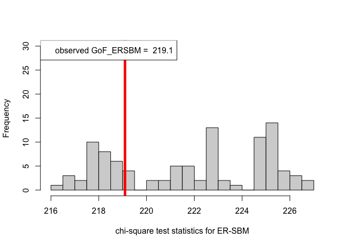
hist(chi_sq_seq.BetaSBM, 20, xlab = "chi-square test statistics for beta-SBM", main = NULL, ylim = c(0, 30))
# adding test statistic on the observed network
abline(v = chi_sq_seq.BetaSBM[1], col = "red", lwd = 5)
legend("topleft", legend = paste("observed GoF_BetaSBM = ", chi_sq_seq.BetaSBM[1]))
From the \(p-\)values obtained viz., \(p_{\mbox{ER-SBM}}, p_{\mbox{beta-SBM}} >> \alpha = 0.05\), we fail to reject the null of a good fit of the given (observed) network to the ER-SBM and beta-SBM, at level \(\alpha = 0.05\).
library(igraph)
RNGkind(sample.kind = "Rounding")
set.seed(1729)

# We model a network with 3 even classes
n1 = 30
n2 = 20
n3 = 50

# Generating block assignments for each of the nodes
n = n1 + n2 + n3
class = rep(c(1, 2, 3), c(n1, n2, n3))

# Generating the adjacency matrix of the network
# Generate the matrix of connection probabilities
cmat = matrix(
  c(
    30, 0.05, 0.05,
    0.05, 30, 0.05,
    0.05, 0.05, 30
  ),
  ncol = 3,
  byrow = TRUE
)
pmat = cmat / n

# Creating the n x n adjacency matrix
adj <- matrix(0, n, n)
for (i in 2:n) {
  for (j in 1:(i - 1)) {
    p = pmat[class[i], class[j]] # We find the probability of connection with the weights
    adj[i, j] = rbinom(1, 1, p) # We include the edge with probability p
  }
}

adjsymm = adj + t(adj)

# When class assignment is known, for ER-SBM
out.ERSBM = goftest_ERSBM(adjsymm, C = class, numGraphs = 100)

# When class assignment is known, for beta-SBM
out.BetaSBM = goftest_BetaSBM(adjsymm, C = class, numGraphs = 100)
#> 2 iterations: deviation 3.353762e-11chi_sq_seq.ERSBM = out.ERSBM$statistic
pvalue.ERSBM = out.ERSBM$p.value
print(pvalue.ERSBM) # p-value in case of the ER-SBM model#> [1] 0.85chi_sq_seq.BetaSBM = out.BetaSBM$statistic
pvalue.BetaSBM = out.BetaSBM$p.value
print(pvalue.BetaSBM) # p-value in case of the beta-SBM model#> [1] 0.04# Plotting histogram of the sequence of the test statistics
hist(chi_sq_seq.ERSBM, 20, xlab = "chi-square test statistics for ER-SBM", main = NULL, ylim = c(0, 30))
# adding test statistic on the observed network
abline(v = chi_sq_seq.ERSBM[1], col = "red", lwd = 5)
legend("topleft", legend = paste("observed GoF_ERSBM = ", chi_sq_seq.ERSBM[1]))
hist(chi_sq_seq.BetaSBM, 20, xlab = "chi-square test statistics for beta-SBM", main = NULL, ylim = c(0, 30))
# adding test statistic on the observed network
abline(v = chi_sq_seq.BetaSBM[1], col = "red", lwd = 5)
legend("topleft", legend = paste("observed GoF_BetaSBM = ", chi_sq_seq.BetaSBM[1]))
Observe that, the \(p-\)value obtained in case of the ER-SBM is muh higher than \(\alpha=0.05\), hence we fail to the reject the null of a good fit of the given (observed) network to the ER-SBM, at level \(\alpha = 0.05\). Whereas, in case of the beta-SBM, the \(p-\)value is nominally smaller than \(\alpha=0.05\), i.e., we weakly reject the null of a good fit of the given (observed) network to the beta-SBM.
Zachary’s Karate Club Data is a classic, well-studied social network of friendships between 34 members of a Karate club at a US university, collected by Wayne Zachary in 1977 (Zachary (1977)).
Here, we consider fitting both the ER-SBM and beta-SBM model with \(k = 2\) blocks, each with sizes \(10\) and \(24\) respectively, i.e., a total of \(n=34\) nodes.
library(igraph)

set.seed(334003213)

data("zachary")

d = zachary # the Zachary's Karate Club data set

# the adjacency matrix
A_zachary = as.matrix(d[1:34, ])
colnames(A_zachary) = 1:34

# obtaining the graph from the adjacency matrix above
g_zachary = igraph::graph_from_adjacency_matrix(A_zachary, mode = "undirected",
                                                weighted = NULL)

# plotting the graph (network) obtained
plot(g_zachary,
main = "Network (Graph) for the Zachary's Karate Club data set")
# block assignments
K = 2 # no. of blocks

n1 = 10
n2 = 24
n = n1 + n2

# known class assignments
class = rep(c(1, 2), c(n1, n2))

# goodness-of-fit tests for the Zachary's Karate Club data set, ER-SBM
out_zachary.ERSBM = goftest_ERSBM(A_zachary, C = class, numGraphs = 100)

chi_sq_seq.ERSBM = out_zachary.ERSBM$statistic
pvalue.ERSBM = out_zachary.ERSBM$p.value
print(pvalue.ERSBM)
#> [1] 0.02# goodness-of-fit tests for the Zachary's Karate Club data set, beta-SBM
out_zachary.BetaSBM = goftest_BetaSBM(A_zachary, C = class, numGraphs = 100)#> 2 iterations: deviation 3.410605e-13chi_sq_seq.BetaSBM = out_zachary.BetaSBM$statistic
pvalue.BetaSBM = out_zachary.BetaSBM$p.value
print(pvalue.BetaSBM)#> [1] 0# Plotting histogram of the sequence of the test statistics
hist(chi_sq_seq.ERSBM, 20, xlab = "chi-square test statistics for ER-SBM", main = NULL, ylim = c(0, 30))
# adding test statistic on the observed network
abline(v = chi_sq_seq.ERSBM[1], col = "red", lwd = 5)
legend("topleft", legend = paste("observed GoF_ERSBM = ", chi_sq_seq.ERSBM[1]))
hist(chi_sq_seq.BetaSBM, 20, xlab = "chi-square test statistics for beta-SBM", main = NULL, ylim = c(0, 30))
# adding test statistic on the observed network
abline(v = chi_sq_seq.BetaSBM[1], col = "red", lwd = 5)
legend("topleft", legend = paste("observed GoF_BetaSBM = ", chi_sq_seq.BetaSBM[1]))
Note that, from the \(p-\)values obtained as well as the observed value of the chi-square test statistic (plotted histograms) under both the framework, i.e., ER-SBM and beta-SBM, we reject the null of a good fit, i.e., the data (network/graph) neither fits to the ER-SBM nor to the beta-SBM; quite similar to the lines of conclusion as claimed by (Karwa et al. (2023)), see Section 7.1.
All of the above examples along with the instances worked-out with the lines of code, deals with the situation where the block assignments are known. On the contrary, if the block assignments \((\mathcal{Z})\) are unknown (with the number of blocks always fixed and known), we refer to (Qin and Rohe (2013)) for estimating the block assignments through regularized spectral clustering. See the following lines of code that is central to the beta-SBM framework.
library(igraph)

set.seed(100)
# goodness-of-fit tests for the Zachary's Karate Club data set;
# with unknown block assignments
out_zachary_unknown = goftest_ERSBM(A_zachary, K = 2, C = NULL, numGraphs = 100)

chi_sq_seq_unknown = out_zachary_unknown$statistic
pvalue_unknown = out_zachary_unknown$p.value
print(pvalue_unknown)
#> [1] 0# Plotting histogram of the sequence of the test statistics
hist(chi_sq_seq_unknown, 20, xlab = "chi-square test statistics", main = NULL, ylim = c(0, 30))
# adding test statistic on the observed network
abline(v = chi_sq_seq_unknown[1], col = "red", lwd = 5)
legend("topleft", legend = paste("observed GoF = ", chi_sq_seq_unknown[1]))
With estimation of the unknown block assignments, the \(p-\)value obtained as well as the observed value of the chi-square test statistic (plotted histogram), similar to the case as shown earlier for known block assignments, we reject the null of a good fit, i.e., the data (network/graph) does not fit the beta-SBM at all.
We would like to thank all the authors of Karwa et al. (2023).