![]()
The goal of ICSClust is to perform tandem clustering
with invariant coordinate selection.
You can install the development version of ICSClust from GitHub with:
# install.packages("devtools")
devtools::install_github("AuroreAA/ICSClust")library(ICSClust)
#> Loading required package: ICS
#> Loading required package: mvtnorm
#> Loading required package: ggplot2
#> Registered S3 method overwritten by 'GGally':
#> method from
#> +.gg ggplot2
# import data
X <- iris[,-5]
# run ICS
ICS_out <- ICS(X)
summary(ICS_out)
#>
#> ICS based on two scatter matrices
#> S1: COV
#> S2: COV4
#>
#> Information on the algorithm:
#> QR: TRUE
#> whiten: FALSE
#> center: FALSE
#> fix_signs: scores
#>
#> The generalized kurtosis measures of the components are:
#> IC.1 IC.2 IC.3 IC.4
#> 1.2074 1.0269 0.9292 0.7405
#>
#> The coefficient matrix of the linear transformation is:
#> Sepal.Length Sepal.Width Petal.Length Petal.Width
#> IC.1 -0.52335 1.9933 2.3731 -4.4308
#> IC.2 0.83296 1.3275 -1.2666 2.7900
#> IC.3 3.05683 -2.2269 -1.6354 0.3654
#> IC.4 0.05244 0.6032 -0.3483 -0.3798
# Pot of generalized eigenvalues
select_plot(ICS_out)
select_plot(ICS_out, type = "lines")
# pairs of all components
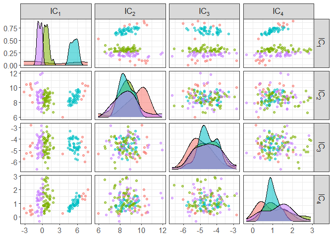
component_plot(ICS_out)
# pairs of only a the first and fourth components
component_plot(ICS_out, select = c(1,4))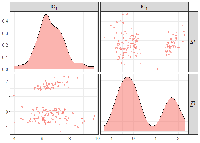
# add some colors by clusters
component_plot(ICS_out, clusters = iris[,5])
component_plot(ICS_out, select = c(1,4), clusters = iris[,5])
# in case you want to do it for initial data
component_plot(X, select = c(1,4), clusters = iris[,5])
# ICSClust requires at least 2 arguments:
# - X: data
# - nb_clusters: nb of clusters
ICS_out <- ICSClust(X, nb_clusters = 3)
summary(ICS_out)
#>
#> ICS based on two scatter matrices
#> S1: COV
#> S2: COV4
#>
#> The generalized kurtosis measures of the components are:
#>   IC.1   IC.2   IC.3   IC.4
#> 1.2074 1.0269 0.9292 0.7405
#>
#> The coefficient matrix of the linear transformation is:
#>      Sepal.Length Sepal.Width Petal.Length Petal.Width
#> IC.1     -0.52335      1.9933       2.3731     -4.4308
#> IC.2      0.83296      1.3275      -1.2666      2.7900
#> IC.3      3.05683     -2.2269      -1.6354      0.3654
#> IC.4      0.05244      0.6032      -0.3483     -0.3798
#>
#>  3 components are selected: IC.4 IC.1 IC.2
#>
#>  3 clusters are identified:
#>
#>  1  2  3
#> 38 62 50
plot(ICS_out)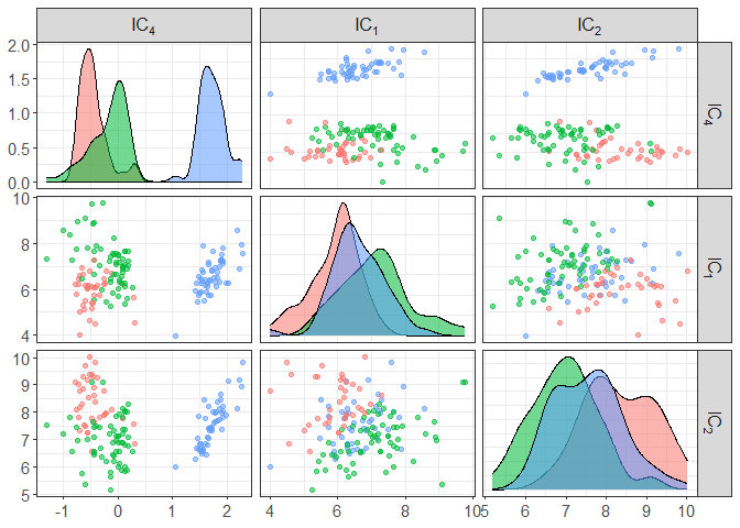
# You can also mention the number of invariant components to keep
ICS_out <- ICSClust(X, nb_select = 2, nb_clusters = 3)
# confusion table with initial clusters
table(ICS_out$clusters, iris[,5])
#>
#>     setosa versicolor virginica
#>   1      0         25        19
#>   2     49          0         0
#>   3      1         25        31
component_plot(ICS_out$ICS_out, select = ICS_out$select, clusters = as.factor(ICS_out$clusters))
# to change the scatter pair
ICS_out <- ICSClust(X, nb_select = 1, nb_clusters = 3,
                ICS_args = list(S1 = ICS_mcd_raw, S2 = ICS_cov,
                                S1_args = list(alpha = 0.5)))
table(ICS_out$clusters, iris[,5])
#>
#>     setosa versicolor virginica
#>   1      0          5        26
#>   2      0         45        24
#>   3     50          0         0
component_plot(ICS_out$ICS_out, clusters = as.factor(ICS_out$clusters))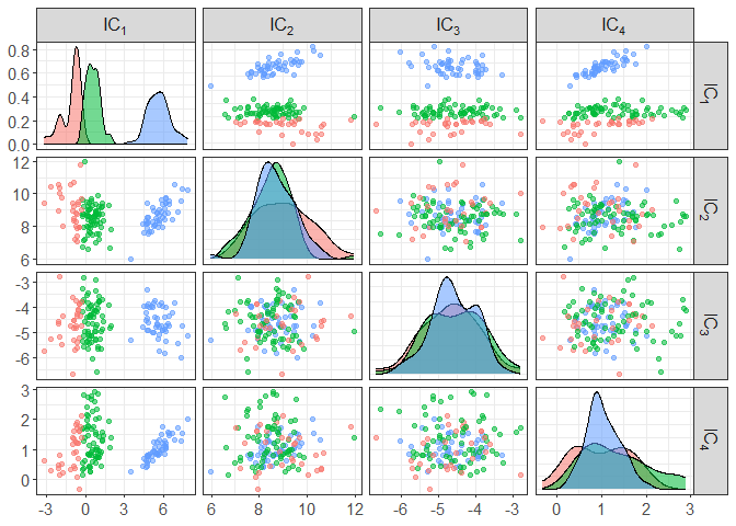
# to change the criteria to select the invariant components
ICS_out <- ICSClust(X, nb_clusters = 3,
                ICS_args = list(S1 = ICS_mcd_raw, S2 = ICS_cov,
                                S1_args = list(alpha = 0.5)),
                criterion = "normal_crit",
                ICS_crit_args = list(level = 0.1, test = "anscombe.test",
                                     max_select = NULL))

component_plot(ICS_out$ICS_out, select = ICS_out$select, clusters = as.factor(ICS_out$clusters))
# to change the clustering method
ICS_out <- ICSClust(X, nb_select = 1, nb_clusters = 3,
                ICS_args = list(S1 = ICS_mcd_raw, S2 = ICS_cov,
                                S1_args = list(alpha = 0.5)),
                method  = "tkmeans_clust",
                clustering_args = list(alpha = 0.1))
table(ICS_out$clusters, iris[,5])
#>
#>     setosa versicolor virginica
#>   0      7          0         8
#>   1      0         40        15
#>   2     43          0         0
#>   3      0         10        27
component_plot(ICS_out$ICS_out, clusters = as.factor(ICS_out$clusters))