![]()
The MR.RGM R package presents a crucial advancement in Mendelian randomization (MR) studies, providing a robust solution to a common challenge. While MR has proven invaluable in establishing causal links between exposures and outcomes, its traditional focus on single exposures and specific outcomes can be limiting. Biological systems often exhibit complexity, with interdependent outcomes influenced by numerous factors. MR.RGM introduces a network-based approach to MR, allowing researchers to explore the broader causal landscape.
With two available functions, RGM and NetworkMotif, the package offers versatility in analyzing causal relationships. RGM primarily focuses on constructing causal networks among response variables and between responses and instrumental variables. On the other hand, NetworkMotif specializes in quantifying uncertainty for given network structures among response variables.
RGM accommodates both individual-level data and two types of summary-level data, making it adaptable to various data availability scenarios. This adaptability enhances the package’s utility across different research contexts. The outputs of RGM include estimates of causal effects, adjacency matrices, and other relevant parameters. Together, these outputs contribute to a deeper understanding of the intricate relationships within complex biological networks, thereby enriching insights derived from MR studies.
You can install MR.RGM R package from CRAN with:
install.packages("MR.RGM")Once the MR.RGM package is installed load the library in the R work-space.
library("MR.RGM")We offer a concise demonstration of the capabilities of the RGM function within the package, showcasing its effectiveness in computing causal interactions among response variables and between responses and instrumental variables using simulated data sets. Subsequently, we provide an example of how NetworkMotif can be applied, utilizing a specified network structure and GammaPst acquired from executing the RGM function.
# Model: Y = AY + BX + E

# Set seed
set.seed(9154)

# Number of data points
n = 10000

# Number of response variables and number of instrument variables
p = 5
k = 6

# Initialize causal interaction matrix between response variables
A = matrix(sample(c(-0.1, 0.1), p^2, replace = TRUE), p, p)

# Diagonal entries of A matrix will always be 0
diag(A) = 0

# Make the network sparse
A[sample(which(A!=0), length(which(A!=0))/2)] = 0

# Create D matrix (Indicator matrix where each row corresponds to a response variable
# and each column corresponds to an instrument variable)
D = matrix(0, nrow = p, ncol = k)

# Manually assign values to D matrix
D[1, 1:2] = 1  # First response variable is influenced by the first 2 instruments
D[2, 3] = 1    # Second response variable is influenced by the 3rd instrument
D[3, 4] = 1    # Third response variable is influenced by the 4th instrument
D[4, 5] = 1    # Fourth response variable is influenced by the 5th instrument
D[5, 6] = 1    # Fifth response variable is influenced by the 6th instrument


# Initialize B matrix
B = matrix(0, p, k)  # Initialize B matrix with zeros

# Calculate B matrix based on D matrix
for (i in 1:p) {
   for (j in 1:k) {
     if (D[i, j] == 1) {
       B[i, j] = 1  # Set B[i, j] to 1 if D[i, j] is 1
     }
   }
 }


# Create variance-covariance matrix
Sigma = 1 * diag(p)

Mult_Mat = solve(diag(p) - A)

Variance = Mult_Mat %*% Sigma %*% t(Mult_Mat)

# Generate instrument data matrix
X = matrix(runif(n * k, 0, 5), nrow = n, ncol = k)

# Initialize response data matrix
Y = matrix(0, nrow = n, ncol = p)

# Generate response data matrix based on instrument data matrix
for (i in 1:n) {

 Y[i, ] = MASS::mvrnorm(n = 1, Mult_Mat %*% B %*% X[i, ], Variance)

}

# Print true causal interaction matrices between response variables and between response and instrument variables
A
#>      [,1] [,2] [,3] [,4] [,5]
#> [1,]  0.0 -0.1  0.0  0.0  0.1
#> [2,]  0.1  0.0 -0.1  0.1  0.1
#> [3,]  0.0 -0.1  0.0  0.0  0.1
#> [4,]  0.0 -0.1  0.0  0.0  0.0
#> [5,]  0.0  0.1  0.0  0.0  0.0
B
#>      [,1] [,2] [,3] [,4] [,5] [,6]
#> [1,]    1    1    0    0    0    0
#> [2,]    0    0    1    0    0    0
#> [3,]    0    0    0    1    0    0
#> [4,]    0    0    0    0    1    0
#> [5,]    0    0    0    0    0    1
We will now apply RGM based on individual level data, summary level data and Beta, SigmaHat matrices to show its functionality.
# Apply RGM on individual level data with Threshold prior
Output1 = RGM(X = X, Y = Y, D = D, prior = "Threshold")

# Calculate summary level data
Syy = t(Y) %*% Y / n
Syx = t(Y) %*% X / n
Sxx = t(X) %*% X / n

# Apply RGM on summary level data for Spike and Slab Prior
Output2 = RGM(Syy = Syy, Syx = Syx, Sxx = Sxx,
           D = D, n = 10000, prior = "Spike and Slab")

# Calculate Beta and Sigma_Hat
# Centralize Data
Y = t(t(Y) - colMeans(Y))
X = t(t(X) - colMeans(X))

# Calculate Sxx
Sxx = t(X) %*% X / n

# Generate Beta matrix and SigmaHat
Beta = matrix(0, nrow = p, ncol = k)
SigmaHat = matrix(0, nrow = p, ncol = k)

for (i in 1:p) {

    for (j in 1:k) {

        fit = lm(Y[, i] ~ X[, j])

        Beta[i, j] =  fit$coefficients[2]

        SigmaHat[i, j] = sum(fit$residuals^2) / n

        }

 }


# Apply RGM on Sxx, Beta and SigmaHat for Spike and Slab Prior
Output3 = RGM(Sxx = Sxx, Beta = Beta, SigmaHat = SigmaHat,
           D = D, n = 10000, prior = "Spike and Slab")
We get the estimated causal interaction matrix between response variables in the following way:
Output1$AEst
#>           [,1]        [,2]       [,3]      [,4]       [,5]
#> [1,] 0.0000000 -0.11032661  0.0000000 0.0000000 0.10676811
#> [2,] 0.0991208  0.00000000 -0.1104576 0.1002182 0.11012341
#> [3,] 0.0000000 -0.09370579  0.0000000 0.0000000 0.09747664
#> [4,] 0.0000000 -0.10185959  0.0000000 0.0000000 0.00000000
#> [5,] 0.0000000  0.10045256  0.0000000 0.0000000 0.00000000
Output2$AEst
#>              [,1]       [,2]          [,3]          [,4]        [,5]
#> [1,]  0.000000000 -0.1127249 -0.0006355133  0.0012237310 0.107520412
#> [2,]  0.099881480  0.0000000 -0.1079853541  0.0996589823 0.109275947
#> [3,] -0.001747246 -0.0929592  0.0000000000 -0.0006473297 0.099778267
#> [4,] -0.003863658 -0.1030056 -0.0024683725  0.0000000000 0.009191016
#> [5,]  0.001966818  0.1014136 -0.0055458038 -0.0050688662 0.000000000
Output3$AEst
#>             [,1]        [,2]         [,3]          [,4]       [,5]
#> [1,]  0.00000000 -0.08972628  0.039412442 -0.0006516754 0.09454632
#> [2,]  0.11040214  0.00000000 -0.112569739  0.0983975424 0.13676682
#> [3,]  0.01896308 -0.09780459  0.000000000  0.0100459671 0.11765744
#> [4,]  0.00000000 -0.11255315  0.001661851  0.0000000000 0.01358832
#> [5,] -0.00174675  0.12947084  0.011533919 -0.0025906139 0.00000000
We get the estimated causal network structure between the response variables in the following way:
Output1$zAEst
#>      [,1] [,2] [,3] [,4] [,5]
#> [1,]    0    1    0    0    1
#> [2,]    1    0    1    1    1
#> [3,]    0    1    0    0    1
#> [4,]    0    1    0    0    0
#> [5,]    0    1    0    0    0
Output2$zAEst
#>      [,1] [,2] [,3] [,4] [,5]
#> [1,]    0    1    0    0    1
#> [2,]    1    0    1    1    1
#> [3,]    0    1    0    0    1
#> [4,]    0    1    0    0    0
#> [5,]    0    1    0    0    0
Output3$zAEst
#>      [,1] [,2] [,3] [,4] [,5]
#> [1,]    0    1    0    0    1
#> [2,]    1    0    1    1    1
#> [3,]    0    1    0    0    1
#> [4,]    0    1    0    0    0
#> [5,]    0    1    0    0    0
We observe that the causal network structures inferred in the three outputs mentioned are identical. To gain a clearer understanding of the network, we compare the true network structure with the one estimated by RGM. Since the networks derived from all three outputs are consistent, we plot a single graph representing the estimated causal network.
# Define a function to create smaller arrowheads
smaller_arrowheads <- function(graph) {
  igraph::E(graph)$arrow.size = 0.60  # Adjust the arrow size value as needed
  return(graph)
}

# Create a layout for multiple plots
par(mfrow = c(1, 2))

# Plot the true causal network
plot(smaller_arrowheads(igraph::graph_from_adjacency_matrix((A != 0) * 1,
       mode = "directed")), layout = igraph::layout_in_circle,
          main = "True Causal Network")

# Plot the estimated causal network
plot(Output1$Graph, main = "Estimated Causal Network")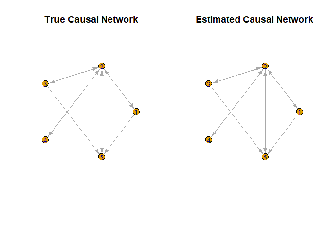
We get the estimated causal interaction matrix between the response and the instrument variables from the outputs in the following way:
Output1$BEst
#>           [,1]     [,2]      [,3]      [,4]      [,5]      [,6]
#> [1,] 0.9921448 1.010301 0.0000000 0.0000000 0.0000000 0.0000000
#> [2,] 0.0000000 0.000000 0.9961312 0.0000000 0.0000000 0.0000000
#> [3,] 0.0000000 0.000000 0.0000000 0.9989298 0.0000000 0.0000000
#> [4,] 0.0000000 0.000000 0.0000000 0.0000000 0.9991987 0.0000000
#> [5,] 0.0000000 0.000000 0.0000000 0.0000000 0.0000000 0.9977224
Output2$BEst
#>           [,1]     [,2]      [,3]      [,4]     [,5]     [,6]
#> [1,] 0.9942219 1.009985 0.0000000 0.0000000 0.000000 0.000000
#> [2,] 0.0000000 0.000000 0.9931885 0.0000000 0.000000 0.000000
#> [3,] 0.0000000 0.000000 0.0000000 0.9992243 0.000000 0.000000
#> [4,] 0.0000000 0.000000 0.0000000 0.0000000 1.000336 0.000000
#> [5,] 0.0000000 0.000000 0.0000000 0.0000000 0.000000 1.001666
Output3$BEst
#>           [,1]     [,2]     [,3]      [,4]      [,5]      [,6]
#> [1,] 0.9910789 1.006024 0.000000 0.0000000 0.0000000 0.0000000
#> [2,] 0.0000000 0.000000 0.993928 0.0000000 0.0000000 0.0000000
#> [3,] 0.0000000 0.000000 0.000000 0.9987596 0.0000000 0.0000000
#> [4,] 0.0000000 0.000000 0.000000 0.0000000 0.9974289 0.0000000
#> [5,] 0.0000000 0.000000 0.000000 0.0000000 0.0000000 0.9948345
We get the estimated graph structure between the response and the instrument variables from the outputs in the following way:
Output1$zBEst
#>      [,1] [,2] [,3] [,4] [,5] [,6]
#> [1,]    1    1    0    0    0    0
#> [2,]    0    0    1    0    0    0
#> [3,]    0    0    0    1    0    0
#> [4,]    0    0    0    0    1    0
#> [5,]    0    0    0    0    0    1
Output2$zBEst
#>      [,1] [,2] [,3] [,4] [,5] [,6]
#> [1,]    1    1    0    0    0    0
#> [2,]    0    0    1    0    0    0
#> [3,]    0    0    0    1    0    0
#> [4,]    0    0    0    0    1    0
#> [5,]    0    0    0    0    0    1
Output3$zBEst
#>      [,1] [,2] [,3] [,4] [,5] [,6]
#> [1,]    1    1    0    0    0    0
#> [2,]    0    0    1    0    0    0
#> [3,]    0    0    0    1    0    0
#> [4,]    0    0    0    0    1    0
#> [5,]    0    0    0    0    0    1
We can plot the log-likelihoods from the outputs in the following way:
plot(Output1$LLPst, type = 'l', xlab = "Iterations", ylab = "Log-likelihood")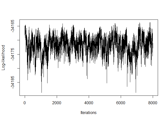
plot(Output2$LLPst, type = 'l', xlab = "Iterations", ylab = "Log-likelihood")
plot(Output3$LLPst, type = 'l', xlab = "Iterations", ylab = "Log-likelihood")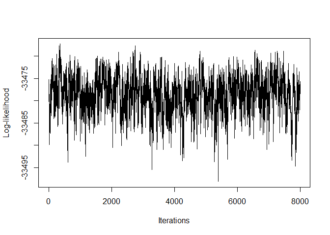
Next, we present the implementation of the NetworkMotif function. We begin by defining a random subgraph among the response variables. Subsequently, we collect GammaPst arrays from various outputs and proceed to execute NetworkMotif based on these arrays.
# Start with a random subgraph
Gamma = matrix(0, nrow = p, ncol = p)
Gamma[5, 2] = Gamma[3, 5] = Gamma[2, 3] = 1

# Plot the subgraph to get an idea about the causal network
plot(smaller_arrowheads(igraph::graph_from_adjacency_matrix(Gamma,
       mode = "directed")), layout = igraph::layout_in_circle,
          main = "Subgraph")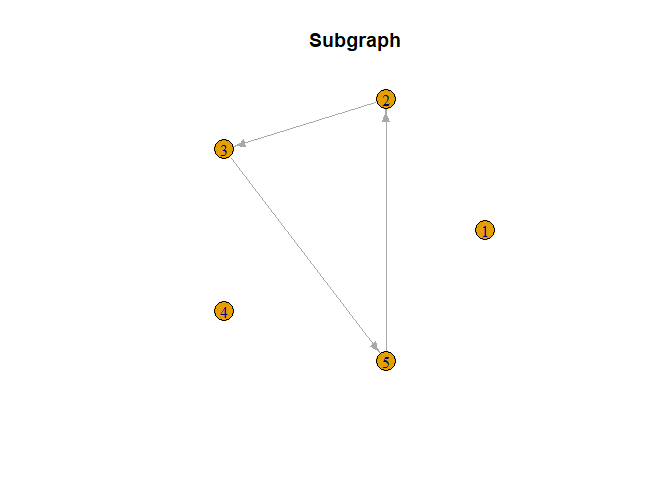
# Store the GammaPst arrays from outputs
GammaPst1 = Output1$GammaPst
GammaPst2 = Output2$GammaPst
GammaPst3 = Output3$GammaPst

# Get the posterior probabilities of Gamma with these GammaPst matrices
NetworkMotif(Gamma = Gamma, GammaPst = GammaPst1)
#> [1] 1
NetworkMotif(Gamma = Gamma, GammaPst = GammaPst2)
#> [1] 0.37325
NetworkMotif(Gamma = Gamma, GammaPst = GammaPst3)
#> [1] 0.461375In real-world scenarios, it is common to encounter a large number of instrumental variables (IVs), each explaining only a small proportion of the trait variance. To better reflect this, we have expanded our simulation setup with the following new elements:
compact_X: By combining
the top PCs from each response variable, we form a condensed matrix
compact_X. This matrix aggregates the instrumental
variables into a more manageable form, facilitating a more efficient
analysis.compact_X, we calculate new summary level data
(Sxx_compact and Syx_compact) for the RGM
function application. This approach provides a more realistic
representation of the instrumental variables’ effects in scenarios with
many IVs explaining only a small proportion of the variance.Here is the updated R code reflecting these changes:
# Load necessary libraries
library(MASS)
library(igraph)
#>
#> Attaching package: 'igraph'
#> The following objects are masked from 'package:stats':
#>
#>     decompose, spectrum
#> The following object is masked from 'package:base':
#>
#>     union

# Set seed for reproducibility
set.seed(9154)

# Number of data points
n = 10000

# Number of response variables
p = 5

# Number of SNPs per response variable
num_snps_per_y = 100

# Total number of SNPs
k = num_snps_per_y * p

# Initialize causal interaction matrix between response variables
A = matrix(sample(c(-0.1, 0.1), p^2, replace = TRUE), p, p)
diag(A) = 0
A[sample(which(A != 0), length(which(A != 0)) / 2)] = 0

# Create D matrix (Indicator matrix where each row corresponds to a response variable
# and each column corresponds to an instrument variable)
D = matrix(0, nrow = p, ncol = k)

# Assign values to D matrix using a loop
for (run in 1:p) {

  D[run, ((run - 1) * 100 + 1) : (run * 100)] = 1

}

# Initialize B matrix
B = matrix(0, p, k)  # Initialize B matrix with zeros

# Calculate B matrix based on D matrix
for (i in 1:p) {
   for (j in 1:k) {
     if (D[i, j] == 1) {
       B[i, j] = 1  # Set B[i, j] to 1 if D[i, j] is 1
     }
   }
 }


# Calculate Variance-Covariance matrix
Sigma = diag(p)
Mult_Mat = solve(diag(p) - A)
Variance = Mult_Mat %*% Sigma %*% t(Mult_Mat)

# Generate instrument data matrix (X)
X = matrix(rnorm(n * k, 0, 1), nrow = n, ncol = k)

# Initialize response data matrix (Y)
Y = matrix(0, nrow = n, ncol = p)

# Generate response data matrix based on instrument data matrix
for (i in 1:n) {
    Y[i, ] = MASS::mvrnorm(n = 1, Mult_Mat %*% B %*% X[i, ], Variance)
}

# Calculate summary level data
Syy = t(Y) %*% Y / n
Syx = t(Y) %*% X / n
Sxx = t(X) %*% X / n

# Perform PCA for each response variable to get top 20 PCs
top_snps_list = list()
for (i in 1:p) {
    X_sub = X[, (num_snps_per_y * (i - 1) + 1):(num_snps_per_y * i)]
    pca = prcomp(X_sub, center = TRUE, scale. = TRUE)
    top_20_pcs = pca$x[, 1:20]
    top_snps_list[[i]] = top_20_pcs
}

# Combine the top PCs from all response variables
compact_X = do.call(cbind, top_snps_list)

# Calculate summary level data based on compact_X
Sxx_compact = t(compact_X) %*% compact_X / n
Syx_compact = t(Y) %*% compact_X / n

# Create D_New
D_New = matrix(0, nrow = p, ncol = 20 * p)

# Assign values to D matrix using a loop
for (run in 1:p) {

  D_New[run, ((run - 1) * 20 + 1) : (run * 20)] = 1

}

# Apply RGM on summary level data for Spike and Slab Prior using the compact_X matrix
Output = RGM(Syy = Syy, Syx = Syx_compact, Sxx = Sxx_compact, D = D_New, n = n, prior = "Spike and Slab")

# Print estimated causal interaction matrices
Output$AEst
#>               [,1]        [,2]         [,3]         [,4]       [,5]
#> [1,]  0.0000000000 -0.10304239  0.012795897  0.006911765 0.09119095
#> [2,]  0.1102430697  0.00000000 -0.101718794  0.095093965 0.10762267
#> [3,] -0.0039579652 -0.10801784  0.000000000 -0.008388722 0.10255348
#> [4,] -0.0013919956 -0.09076408  0.011536478  0.000000000 0.01075220
#> [5,] -0.0005533104  0.10848253 -0.002160112 -0.011725145 0.00000000
Output$zAEst
#>      [,1] [,2] [,3] [,4] [,5]
#> [1,]    0    1    0    0    1
#> [2,]    1    0    1    1    1
#> [3,]    0    1    0    0    1
#> [4,]    0    1    0    0    0
#> [5,]    0    1    0    0    0

# Create a layout for multiple plots
par(mfrow = c(1, 2))

# Plot the true causal network
plot(smaller_arrowheads(igraph::graph_from_adjacency_matrix((A != 0) * 1, mode = "directed")),
     layout = igraph::layout_in_circle, main = "True Causal Network")

# Plot the estimated causal network
plot(Output$Graph, main = "Estimated Causal Network")
Conclusion
Although we have mimicked a real-world setup where there are numerous instrumental variables (IVs), each explaining only a small portion of the trait variance, our approach still yields very promising results. This demonstrates that our method is robust even in complex scenarios with many IVs.
The dimensionality reduction technique we employed, specifically using Principal Component Analysis (PCA) to select the top principal components as IVs, proves to be effective. This approach can be broadly applied to similar problems where dimensionality reduction is necessary. By leveraging PCA or other dimensionality reduction methods, researchers can efficiently manage large sets of IVs and apply our algorithm to gain valuable insights into causal relationships.
Yang Ni. Yuan Ji. Peter Müller. “Reciprocal Graphical Models for Integrative Gene Regulatory Network Analysis.” Bayesian Anal. 13 (4) 1095 - 1110, December 2018. https://doi.org/10.1214/17-BA1087