coverR2

Package coveR2 allows to import, classify and analyze Digital Cover Photography (DCP) images of tree canopies and export forest canopy attributes like Foliage Cover and Leaf Area Index (LAI).

The DCP method was pioneered by Macfarlane et al. 2007a, and it is based in acquiring upward-looking images of tree crowns using a normal lens, namely a lens with a restricted (typically 30°) field of view (FOV), although larger FOV images (e.g. those from camera traps or smartphones) can be considered.

The process of analyzing these images is substantially:
1) import a cover image;
2) create a binary image of canopy (0) and gaps (1);
3) further classify gaps based on their size (large and small gaps);
4) apply theoretical gap formulas to relate canopy structure to gap fraction.

Installation

The coveR2 package is a wrapper of the coveR (Chianucci et al. 2022) package which is available only as development version here. To make the package available in CRAN, coveR2 has not reading-EXIF functionality, which avoids third-party software needs.

The coveR2 can be installed from CRAN:

install.packages('coveR2')

A development version is available from GitLab:

# install.packages("devtools")
devtools::install_gitlab("fchianucci/coveR2")

Workflow

The basic steps of processing cover images are:

1. import an image
2. create a binary classification of gaps and canopy
3. label each gap
4. classify gaps based on their size
5. retrieve canopy attributes from gap size

All these steps are performed by a single function coveR2(). The following sections illustrate step-by-step the whole workflow required to retrieve canopy attributes from DCP images.

1) Open an image and select the blue-channel.

First we need to import an RGB image:

library(coveR2)
image <- system.file('extdata','IMG1.JPG',package='coveR2')

The first step of the coveR2 function allows to import the image as a single-channel raster, using terra::rast(band=x) functionality. The blue channel coveR2(filename, channel=3) is generally preferred as it enables highest contrast between sky and canopy pixels, easing image classification. This is well illustrated in the following figure:

We can then take the blue channel image using the channel=3 argument:

The extra-argument crop allows to specify if some horizontal lines should be removed from the bottom side of the image. This option is useful when removing the timestamp from camera trap images. These data are useful when the method is applied to continuous cameras, such as camera traps, see Chianucci et al. (2021).

2) Classify and create a binary raster image.

Once imported, the functions uses the thdmethod argument to classify the blue-channel pixels to get a binary image of sky (1) and canopy (0) pixels. Note that the sky (hereafter gap) pixels are the target of subsequent analyses.

coveR2 function uses the auto_thresh() functionality of the autothresholdr package (Landini et al. 2017) to define an image threshold. The default thresholding function used by thd_blue is ‘Otsu’. For other methods, see: https://imagej.net/plugins/auto-threshold

After this steps, a single channel binary (0,1) SpatRaster is created, which can be inspected with the display extra-argument:

3) Segment and create labelled gaps image.

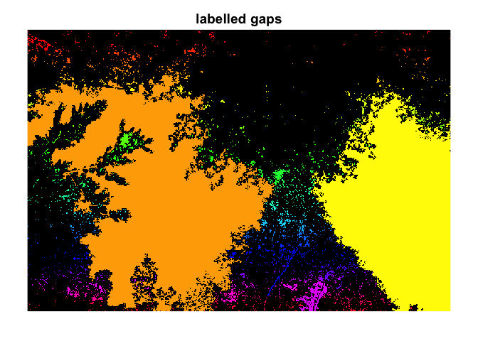
Retrieving canopy attributes requires further classifying gap pixels (those labelled as 1 in the binary raster image) as large, between-crowns gaps and small, within-crown gaps. The function use the ConnCompLabel functionality of mcg package (https://cran.r-project.org/package=mgc) to assign a numeric label to each distinct gap.

The function returns a single-channel raster image with each gap with a numeric unique label:

Once labelled, each gaps can be classified based on their size.

4) Classify gaps based on their size.

There are basically two methods to classify gaps based on their (pixel) size. A very effective method is the one proposed by Macfarlane et al. 2007b which consider large gaps (gL) those larger 1.3% of the image area (this value can be varied in the thd argument). It can be selected via the gapmethod='macfarlane' argument.

Alternatively, we can use the large gap method proposed by Alivernini et al. 2018 which is based on the statistical distribution of gap size inside images. In this method large gaps (gL) are considers as: \(gL \ge \mu + \sqrt{{\sigma \over n}}\). Compared with the other method, this is canopy-density dependent, as the large gap threshold varied with the actual canopy considered. It can be selected via the gapmethod='alivernini' argument.

#>   Var1   Freq     id     NR        gL
#> 1    0 432282 IMG1_3 763264    Canopy
#> 2    1      1 IMG1_3 763264 Small_gap
#> 3    2    319 IMG1_3 763264 Small_gap
#> 4    3   1768 IMG1_3 763264 Small_gap
#> 5    4     12 IMG1_3 763264 Small_gap
#> 6    5      1 IMG1_3 763264 Small_gap

The function returns a dataframe of classified pixels into ‘Canopy’, ‘Small_gap’ and ‘Large_gap’ classes. ‘Var1’>0 identify each gap region, ‘Freq’ is the number of pixels in each gap, while ‘NR’ is the image size.

5) Retrieving canopy attributes from classified gap and canopy pixels

Once we classified gaps into large and small gaps using one of the two methods above, the coveR function estimates canopy attributes from the following modified Beer-Lambert law equations Macfarlane et al. 2007a. The inversion for leaf area requires parametrizing an extinction coefficient k, which is by default set to 0.5 (spherical leaf angle distribution):

• Gap fraction (GF) is calculated as the fraction of gap pixels (those labelled as 1 in the binary image):

  \[ GF= {gT \over NR} \]

  where \(gT\) is the number of gap pixels, \(NR\) is the total number of image pixels.;

• Foliage Cover (FC) is the complement of gap fraction:

  \[ FC= 1-GF \]

• Crown Cover (CC) is calculated as the complement of large gap fraction:

  \[CC= 1-{gL \over NR}\], where \(gL\) is the number of large gap pixels, \(NR\) is the total number of image pixels;

• Crown Porosity (CP) is calculated as the fraction of gaps within crown envelopes:

\[ CP=1- {FC \over CC} \]

By knowing these canopy attributes, it is possible to derive effective LAI (Le) as:

\[ Le= {-log(GF) \over k} \]

• The actual LAI (L) is calculated as:

\[ L=-CC {log(CP) \over k} \]

As the actual LAI considers clumping effects, \(L \ge Le\).

• the Clumping Index (CI) is calculated as:

\[ CI = {Le \over L} \]

#> # A tibble: 1 × 12
#>   id          FC    CC     CP    Le     L    CI     k imgchannel gapmethod 
#>   <chr>    <dbl> <dbl>  <dbl> <dbl> <dbl> <dbl> <dbl>      <dbl> <chr>     
#> 1 IMG1.JPG 0.565 0.604 0.0646 0.980  1.95 0.503  0.85          3 macfarlane
#> # ℹ 2 more variables: imgmethod <chr>, thd <dbl>

6) Export the classified image

We can export the raster image with classified gap sizes using the export.image argument function.

More about

The functions are optimized to batch processing bunches of DCP images. In such a case, you can use ‘traditional’ looping through images, as in example below.

data_path<-system.file('extdata',package='coveR2')
files<-dir(data_path,pattern='jpeg$|JPG$', full.names = T)

res<-NULL
for (i in 1:length(files)){
  cv<-coveR2(files[i], display=F, message=F)
  res<-rbind(res,cv)
}

res
#> # A tibble: 2 × 12
#>   id          FC    CC     CP    Le     L    CI     k imgchannel gapmethod 
#>   <chr>    <dbl> <dbl>  <dbl> <dbl> <dbl> <dbl> <dbl>      <dbl> <chr>     
#> 1 IMG1.JPG 0.565 0.604 0.0646  1.67  3.31 0.503   0.5          3 macfarlane
#> 2 IMG3.JPG 0.711 0.777 0.0847  2.48  3.83 0.647   0.5          3 macfarlane
#> # ℹ 2 more variables: imgmethod <chr>, thd <dbl>

References

Alivernini, A., Fares, S., Ferrara, C. and Chianucci, F., 2018. An objective image analysis method for estimation of canopy attributes from digital cover photography. Trees, 32, pp.713-723. https://doi.org/10.1007/s00468-018-1666-3

Chianucci, F., Bajocco, S. and Ferrara, C., 2021. Continuous observations of forest canopy structure using low-cost digital camera traps. Agricultural and Forest Meteorology, 307, p.108516. https://doi.org/10.1016/j.agrformet.2021.108516

Chianucci, F., Ferrara, C. and Puletti, N., 2022. coveR: an R package for processing digital cover photography images to retrieve forest canopy attributes. Trees, 36(6), pp.1933-1942. https://doi.org/10.1007/s00468-022-02338-5

Landini, G., Randell, D.A., Fouad, S. and Galton, A., 2017. Automatic thresholding from the gradients of region boundaries. Journal of microscopy, 265(2), pp.185-195. https://doi.org/10.1111/jmi.12474

Macfarlane, C., Hoffman, M., Eamus, D., Kerp, N., Higginson, S., McMurtrie, R. and Adams, M., 2007a. Estimation of leaf area index in eucalypt forest using digital photography. Agricultural and forest meteorology, 143(3-4), pp.176-188. https://doi.org/10.1016/j.agrformet.2006.10.013

Macfarlane, C., Grigg, A. and Evangelista, C., 2007b. Estimating forest leaf area using cover and fullframe fisheye photography: thinking inside the circle. Agricultural and Forest Meteorology, 146(1-2), pp.1-12. https://doi.org/10.1016/j.agrformet.2007.05.001