Marlon E. Cobos, Hannah L. Owens, Jorge Soberón, A. Townsend Peterson
![]()
The package mop contains a set of tools to perform the Mobility Oriented-Parity (MOP) metric, which helps to compare a set of conditions of reference versus another set of of interest. The main goals of the MOP metric are to explore conditions in the set of interest that are non-analogous to those in the reference set, and to quantify how different conditions in the set of interest are. The tools included here help to identify conditions outside the rages of the reference set with greater detail than in earlier implementations. These tools are based on the methods proposed by Owens et al. (2013).
To install the stable version of mop use:
Before installing the development version of mop, make sure to obtain the compilation tools required: Rtools for Windows, Xcode for Mac, and ggc or similar compilers in Linux, see examples here or here.
After that, you can install the development version of mop from its GitHub repository with:
The following are basic examples of how to use the main function of the package. First, load the package and some example data.
# package
library(mop)
# data
## current conditions
reference_layers <- terra::rast(system.file("extdata", "reference_layers.tif",
package = "mop"))
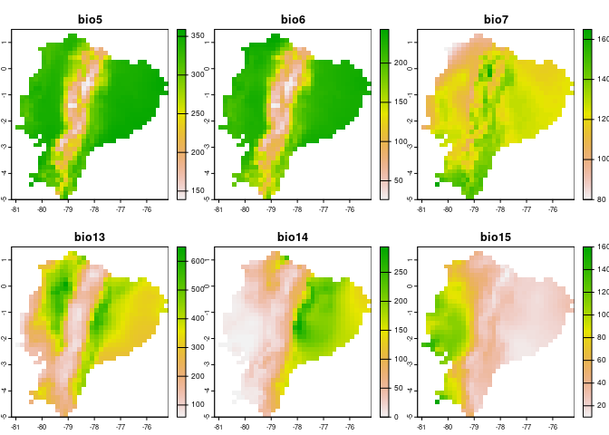
## future conditions
layers_of_interest <- terra::rast(system.file("extdata",
"layers_of_interest.tif",
package = "mop"))
# plot the data
## variables to represent current conditions
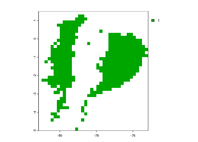
terra::plot(reference_layers)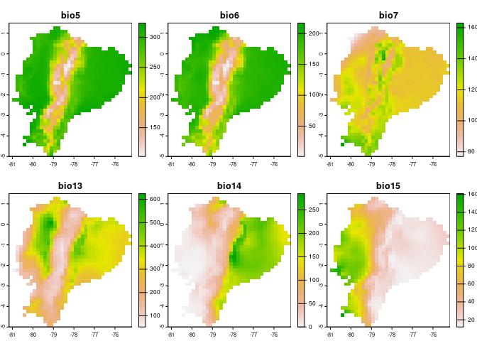
The code below helps to run analyses with all the details implemented in the function. To see more basic options and what they imply, check the function documentation with help(mop). Parallel processing is allowed via arguments of this function.
# analysis
mop_basic_res <- mop(m = reference_layers, g = layers_of_interest,
                     type = "detailed", calculate_distance = TRUE,
                     where_distance = "all", distance = "euclidean",
                     scale = TRUE, center = TRUE)
#>   |                                                                              |                                                                      |   0%  |                                                                              |===================================                                   |  50%  |                                                                              |======================================================================| 100%

# summary
summary(mop_basic_res)
#>
#>                         Summary of MOP resuls
#> ---------------------------------------------------------------------------
#>
#> MOP summary:
#> Values
#>       type scale center calculate_distance  distance percentage
#> 1 detailed  TRUE   TRUE               TRUE euclidean          1
#>   rescale_distance fix_NA N_m N_g
#> 1            FALSE   TRUE 723 723
#>
#> Reference conditions
#>           bio5       bio6      bio7     bio13     bio14     bio15
#> min -3.1625758 -2.8057083 -3.609429 -2.002072 -1.170877 -1.027498
#> max  0.6507328  0.8513394  3.710556  2.779598  2.351446  3.174031
#>
#>
#> Distances:
#>       min      mean       max
#> 0.3003245 0.9373088 2.1788036
#>
#>
#> Non-analogous conditions (NAC):
#> Percentage = 0.566% of all contions
#> Variables with NAC in 'simple' = 2
#>
#>
#> Detailed results were obtained, not shown here

# print results
mop_basic_res
#> MOP distances:
#> class       : SpatRaster
#> dimensions  : 39, 36, 1  (nrow, ncol, nlyr)
#> resolution  : 0.1666667, 0.1666667  (x, y)
#> extent      : -81.16667, -75.16667, -5, 1.5  (xmin, xmax, ymin, ymax)
#> coord. ref. : lon/lat WGS 84 (with axis order normalized for visualization)
#> source(s)   : memory
#> name        :       mop
#> min value   : 0.3003245
#> max value   : 2.1788036
#>
#> MOP basic:
#> class       : SpatRaster
#> dimensions  : 39, 36, 1  (nrow, ncol, nlyr)
#> resolution  : 0.1666667, 0.1666667  (x, y)
#> extent      : -81.16667, -75.16667, -5, 1.5  (xmin, xmax, ymin, ymax)
#> coord. ref. : lon/lat WGS 84 (with axis order normalized for visualization)
#> source(s)   : memory
#> name        : mop
#> min value   :   1
#> max value   :   1
#>
#> MOP simple:
#> class       : SpatRaster
#> dimensions  : 39, 36, 1  (nrow, ncol, nlyr)
#> resolution  : 0.1666667, 0.1666667  (x, y)
#> extent      : -81.16667, -75.16667, -5, 1.5  (xmin, xmax, ymin, ymax)
#> coord. ref. : lon/lat WGS 84 (with axis order normalized for visualization)
#> source(s)   : memory
#> categories  : n_variables
#> name        : n_variables
#> min value   :           1
#> max value   :           2
#>
#> MOP detailed:
#> interpretation_combined:
#>   values extrapolation_variables
#> 1  1e+01                    bio5
#> 2  1e+02                    bio6
#> 3  1e+03                    bio7
#> 4  1e+04                   bio13
#> 5  1e+05                   bio14
#> 6  1e+06                   bio15
#> ...
#>
#> towards_low_end:
#> class       : SpatRaster
#> dimensions  : 39, 36, 6  (nrow, ncol, nlyr)
#> resolution  : 0.1666667, 0.1666667  (x, y)
#> extent      : -81.16667, -75.16667, -5, 1.5  (xmin, xmax, ymin, ymax)
#> coord. ref. : lon/lat WGS 84 (with axis order normalized for visualization)
#> source(s)   : memory
#> names       : bio5, bio6, bio7, bio13, bio14, bio15
#> min values  :  NaN,  NaN,  NaN,   NaN,   NaN,     1
#> max values  :  NaN,  NaN,  NaN,   NaN,   NaN,     1
#>
#> towards_high_end:
#> class       : SpatRaster
#> dimensions  : 39, 36, 6  (nrow, ncol, nlyr)
#> resolution  : 0.1666667, 0.1666667  (x, y)
#> extent      : -81.16667, -75.16667, -5, 1.5  (xmin, xmax, ymin, ymax)
#> coord. ref. : lon/lat WGS 84 (with axis order normalized for visualization)
#> source(s)   : memory
#> names       : bio5, bio6, bio7, bio13, bio14, bio15
#> min values  :    1,    1,    1,     1,     1,   NaN
#> max values  :    1,    1,    1,     1,     1,   NaN
#>
#> towards_low_combined:
#> class       : SpatRaster
#> dimensions  : 39, 36, 1  (nrow, ncol, nlyr)
#> resolution  : 0.1666667, 0.1666667  (x, y)
#> extent      : -81.16667, -75.16667, -5, 1.5  (xmin, xmax, ymin, ymax)
#> coord. ref. : lon/lat WGS 84 (with axis order normalized for visualization)
#> source(s)   : memory
#> categories  : extrapolation_variables
#> name        : extrapolation_variables
#> min value   :                   bio15
#> max value   :                   bio15
#>
#> towards_high_combined:
#> class       : SpatRaster
#> dimensions  : 39, 36, 1  (nrow, ncol, nlyr)
#> resolution  : 0.1666667, 0.1666667  (x, y)
#> extent      : -81.16667, -75.16667, -5, 1.5  (xmin, xmax, ymin, ymax)
#> coord. ref. : lon/lat WGS 84 (with axis order normalized for visualization)
#> source(s)   : memory
#> categories  : extrapolation_variables
#> name        : extrapolation_variables
#> min value   :                    bio5
#> max value : bio14Below are some example plots of the results that can be obtained from analysis with mop.
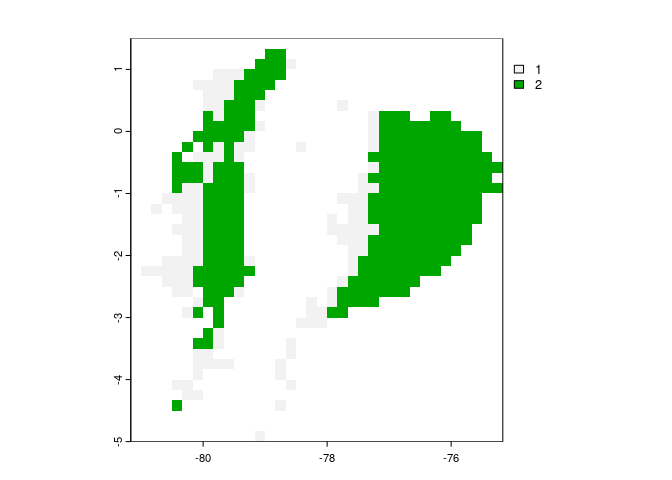
# difference between set of conditions of interest and the reference set
terra::plot(mop_basic_res$mop_distances)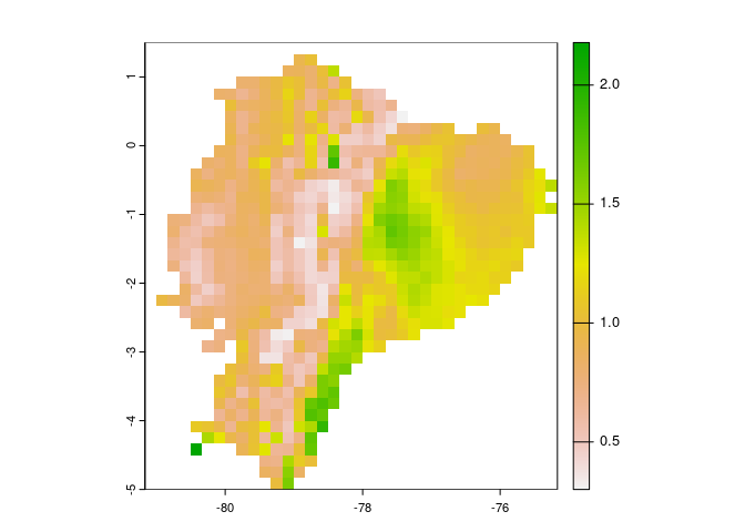
# combinations of variables with non-analogous conditions towards high values
terra::plot(mop_basic_res$mop_detailed$towards_high_combined)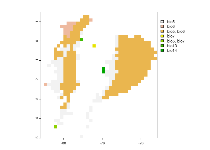
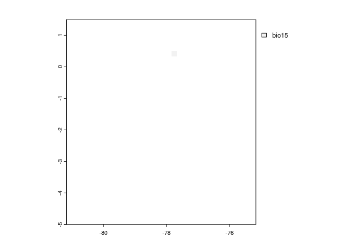
# combinations of variables with non-analogous conditions towards low values
terra::plot(mop_basic_res$mop_detailed$towards_low_combined)