
ravetools is the signal- and image-processing toolbox
behind RAVE, a software suite for analyzing
intracranial Electroencephalography (iEEG)
data.
It is deliberately a mathematical toolbox rather than an analysis
pipeline. It supplies the fast, memory-efficient primitives - filters,
spectral decomposition, image registration, surface geometry - and
leaves the user-facing pipelines to the other RAVE packages
built on top of it. Every routine is a plain function operating on plain
R objects.
Highlights:
Notch filter, Welch
periodogram, and Morlet wavelet that scale to hours of
high-resolution recordingCARLA
re-referencing, canonical response parameterization, and basis profile
curvesFIR and IIR filter design driven by a
specification instead of a filter order, with stability diagnosticsrigid,
affine, and SyN) that depends on no external
registration libraryrgl
dependencyC++ array primitives and direct access to
FFTW3| Part | Contents |
|---|---|
| 1. Signal processing | Channel diagnosis and time-frequency decomposition; brain stimulation tools; filter design |
| 2. Image processing | 3D volume registration and resampling; surface reconstruction and rendering; low-level geometry |
| 3. Utilities and helpers | FFTW3 bindings, parallel
array operations, geometry classes, binary readers |
The complete function reference lives at dipterix.org/ravetools.
The package is on CRAN. To install the compiled version,
simply run:
install.packages("ravetools")Development builds are on r-universe:
install.packages("ravetools", repos = "https://dipterix.r-universe.dev")Installing from source needs a C++ compiler, the FFTW3 library, and
pkg-config - nothing else. See this
document for platform-by-platform instructions.
The starting point for a channel is usually to look at it, clean the line noise, and decompose it in time and frequency.
Generate a toy channel and inspect it. diagnose_channel
combines the trace, the Welch periodogram, and the
histogram into one figure:
library(ravetools)
set.seed(2023)

# Generate 20 second data at 2000 Hz
time <- seq(0, 20, by = 1 / 2000)
signal <- sin( 120 * pi * time) +
  sin(time * 20*pi) +
  exp(-time^2) *
  cos(time * 10*pi) +
  rnorm(length(time))

diagnose_channel(signal, srate = 2000)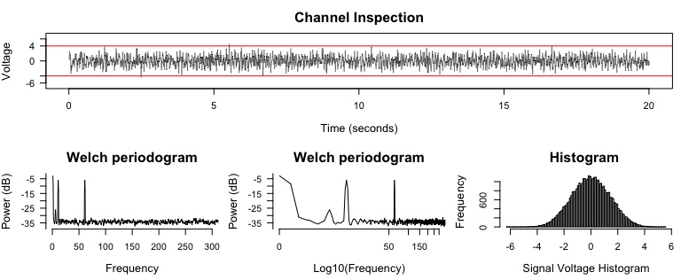
notch_filter removes the electrical line frequency and
its harmonics. Passing two signals to diagnose_channel
compares them side by side:
## ------- Notch filter --------
signal2 <- notch_filter(signal, sample_rate = 2000)

diagnose_channel(signal, signal2, srate = 2000,
                 name = c("Raw", "Filtered"))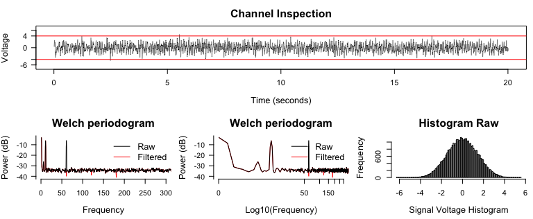
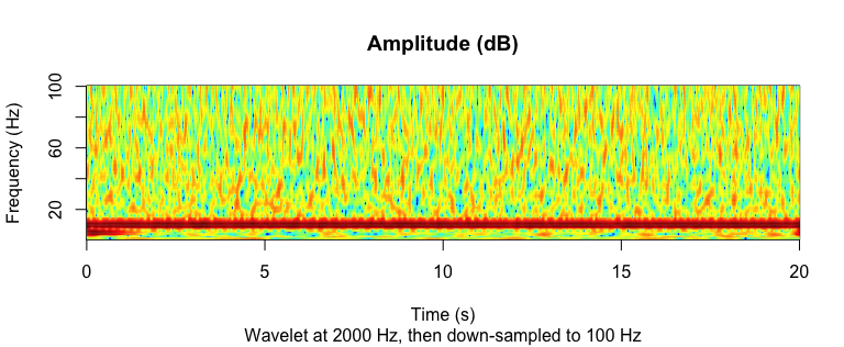
There are two ways to obtain a time-frequency decomposition.
morlet_wavelet uses the Morlet wavelet
and returns both amplitude and phase; multitaper returns no
phase, but its amplitude is smoother.
Using morlet_wavelet:
## ---------- Wavelet -----------
coef <- morlet_wavelet(
  signal2, freqs = seq(1, 100, by = 1),
  srate = 2000, wave_num = c(2, 15))
amplitude <- 20 * log10(Mod(coef[]))

# For each frequency, decimate to 100 Hz
downsample_amp <- apply(amplitude, 2, decimate, q = 20)
downsample_time <- decimate(time, q = 20)

par(mfrow = c(1,1))
image(
  z = downsample_amp,
  x = downsample_time,
  y = seq(1, 100, by = 1),
  xlab = "Time (s)",
  ylab = "Frequency (Hz)",
  main = "Amplitude (dB)",
  sub = "Wavelet at 2000 Hz, then down-sampled to 100 Hz",
  col = matlab_palette()
)
For very long recordings,
morlet_wavelet(segment_length = ...) processes the signal
in overlapping segments, cutting peak memory and FFT cost
without changing the result on the signal interior.
Using multitaper. The algorithm is modified from source
code here;
please credit them as well if you adopt this approach.
## ---------- Multitaper -----------
res <- multitaper(
  data = signal2,
  fs = 2000,
  frequency_range = c(1, 100),
  time_bandwidth = 5,
  window_params = c(2, 0.05)
)

par(mfrow = c(1,1))
image(
  x = res$time,
  y = res$frequency,
  z = 10 * log10(res$spec),
  xlab = "Time (s)",
  ylab = 'Frequency (Hz)',
  col = matlab_palette(),
  main = "Amplitude (dB)"
)
Also in this group: pwelch and mv_pwelch
for power spectral density, plot_signals for drawing many
traces on one canvas, baseline_array for baseline
correction across array margins (seven methods, including decibel and
z-score), plus decimate, detrend,
find_peaks, gammatone_fast,
wavelet_kernels, and
wavelet_cycles_suggest.
Single-pulse electrical stimulation produces cortico-cortical evoked
potentials (CCEPs). ravetools implements three
published methods for analyzing them. Each is a faithful
re-implementation, so please cite the original work if you use it.
carla selects the subset of channels
that makes the cleanest common average reference, by choosing the subset
size with the least anti-correlation against the remaining channels.
From Huang and colleagues (2024), doi:10.1016/j.jneumeth.2024.110153;
the virtual_reference = TRUE variant follows Huang and
colleagues (2025), doi:10.1016/j.jneumeth.2025.110461.
crp parameterizes single-trial evoked
responses: it estimates the response duration, extracts the canonical
response shape, and reports per-trial weights, signal-to-noise, and
explained variance. From Miller and colleagues (2023), doi:10.1371/journal.pcbi.1011105.
bpc identifies a small set of basis
profile curves shared across stimulation sites, then assigns each site
to the curve that best explains its trials. From Miller and colleagues
(2021), doi:10.1371/journal.pcbi.1008710.
A basic run through the first two:
set.seed(42)

# A toy CCEP epoch: 16 channels x 30 trials, only channels 1-4 respond
sample_rate <- 1000
time <- seq(-0.1, 0.4 - 1 / sample_rate, by = 1 / sample_rate)
nchan <- 16
ntrial <- 30
evoked <- ifelse(time >= 0, 80 * exp(-time / 0.05) * sin(2 * pi * 12 * time), 0)

x <- array(rnorm(length(time) * ntrial * nchan, sd = 5),
           dim = c(length(time), ntrial, nchan))
for (ch in 1:4) {
  for (k in seq_len(ntrial)) {
    x[, k, ch] <- x[, k, ch] + evoked * runif(1, 0.6, 1.4)
  }
}

# 1. Which channels make the cleanest common average reference?
#    `x` is time x trials x channels, cropped to the responsive window.
fit <- carla(x[time > 0 & time <= 0.3, , , drop = FALSE])
fit$n_optimum   #> 12
fit$channels    #> 5 6 7 8 9 10 11 12 13 14 15 16   (channels 1-4 excluded)

# 2. Re-reference against that subset
reference <- apply(x[, , fit$channels, drop = FALSE], c(1, 2), mean)
x_ref <- sweep(x, c(1, 2), reference, "-")

# 3. Parameterize the evoked response on a responsive channel
res <- crp(x_ref[, , 1], time = time, t_start = 0.015, t_end = 0.3)
res$tau_R       #> 0.119   (response duration, in seconds)

plot(res)
carla also accepts a filearray in place of
an in-memory array, so large datasets can stay on disk.
For continuous stimulation rather than single pulses,
stimpulse_find, stimpulse_align,
stimpulse_extract, and stimpulse_interpolate
locate the pulse train, align the pulses, and interpolate the artifact
away. The bundled stimulation_signal dataset is a
one-second recording at 30 kHz to try them on.
Most filtering work starts from a specification - a pass band of 8 to
12 Hz, fully attenuated beyond 6 and 14 Hz - rather than from a filter
order. design_filter takes that specification and, given
data, designs and applies the filter in a single call:
filtered <- design_filter(
  data = signal, sample_rate = 2000,
  high_pass_freq = 8, low_pass_freq = 12
)
design_filter_fir and design_filter_iir
return the filter itself, so it can be inspected before being committed
to. diagnose_filter draws the pass band, the stop band, the
phase response, and the effect on a sample signal in one figure:
set.seed(1)
sample_rate <- 200
time <- seq(0, 10, by = 1 / sample_rate)

# A mixture of 2 Hz, 10 Hz, and 60 Hz
x <- sin(time * 4 * pi) + sin(time * 20 * pi) +
  2 * sin(time * 120 * pi) + rnorm(length(time), sd = 0.4)

# Design an alpha-band filter from the specification rather than from an order
filter <- design_filter_fir(
  sample_rate = sample_rate,
  high_pass_freq = 8, high_pass_trans_freq = 2,
  low_pass_freq = 12, low_pass_trans_freq = 2
)
filter          #> <FIR filter>   Method: kaiser   Order: 223

# Inspect the filter against the signal it will be applied to
diagnose_filter(filter$b, filter$a, fs = sample_rate, sample = x)
IIR filters can be numerically unstable at high orders,
so design_filter checks the order it derives against
rcond_filter_ar, the reciprocal condition number of the
autoregressive coefficients, and check_filter reports the
achieved magnitude at any frequency. The filter printed above carries
both.
Also in this group: filter_signal and
filtfilt for applying filters (filtfilt
accepts a gsignal second-order-section object),
freqz2 for the frequency response, band_pass1
and band_pass2, the fir1 and
firls designers, and the window functions
hamming, hanning, blackman,
blackmanharris, blackmannuttall,
bohmanwin, and flattopwin.
The classical analog prototype designers - butter,
cheby1, cheby2, ellip, and their
order-selection companions - are re-exported from gsignal
for convenience. They belong to that package, not to this one.
register_volume3d aligns two 3D volumes: CT
to MRI, MRI to MRI, or a subject
to a template. It is implemented from scratch in RcppEigen
and mirrors the behavior of ANTs
antsRegistration - a multi-resolution,
physical-shift-scaled gradient-descent optimizer driving a similarity
metric, working entirely in anatomical RAS space. It
depends on no external registration library.
Each volume carries its own vox2ras matrix, so volumes
differing in sampling, orientation, or field of view are handled
correctly. The transform can be rigid (6 degrees of
freedom), affine (12), or syn (an
affine followed by a symmetric diffeomorphic
deformation).
The example below is self-contained: it displaces a known volume by a known transform, then recovers it.
data("left_hippocampus_mask")

# Blur the binary mask into a smooth intensity volume, and place it in RAS
gauss3 <- function(n = 5, sigma = 1.2) {
  g <- exp(-(seq(-(n - 1) / 2, (n - 1) / 2)^2) / (2 * sigma^2))
  array(outer(outer(g, g), g), dim = c(n, n, n)) / sum(g)^3
}
target <- convolve_volume(left_hippocampus_mask, gauss3())
vox2ras <- diag(4)
vox2ras[1:3, 4] <- -dim(target) / 2

# A known displacement: 8 degrees about the z axis, plus a translation
theta <- 8 * pi / 180
known <- diag(4)
known[1:2, 1:2] <- c(cos(theta), sin(theta), -sin(theta), cos(theta))
known[1:3, 4] <- c(2.5, -3, 1.5)

# Resample the target through the inverse to obtain a misaligned source
source <- apply_transform3d(target, vox2ras, solve(known))

# Recover the displacement
aligned <- register_volume3d(
  source, target,
  source_vox2ras = vox2ras, target_vox2ras = vox2ras,
  type = "syn", metric = "cc", verbose = FALSE
)
round(aligned$transform[1:3, 4], 2)   #> 2.51 -3.04 1.49   (known: 2.5 -3 1.5)

slice <- 22
zlim <- range(target)
pal <- grDevices::grey.colors(256, start = 0, end = 1)
oldpar <- par(mfrow = c(1, 4), mar = c(0.5, 0.5, 2.5, 0.5))
image(target[, , slice], asp = 1, axes = FALSE, col = pal, zlim = zlim,
      main = "Target (fixed)")
image(source[, , slice], asp = 1, axes = FALSE, col = pal, zlim = zlim,
      main = "Source (moving)")
image(aligned$image[, , slice], asp = 1, axes = FALSE, col = pal, zlim = zlim,
      main = "Aligned")
image(abs(aligned$image - target)[, , slice], asp = 1, axes = FALSE, col = pal,
      zlim = zlim, main = "Absolute difference")
par(oldpar)
The result carries the 4x4 RAS-to-RAS
transform, the warped image, and, for
syn, the forward_field and
inverse_field deformations. apply_transform3d
replays any of them onto a new volume.
register_volume3d accepts more than one modality: pass a
list of co-registered volumes with per-channel
weights and metric to let a T1, a
T2, and an atlas jointly drive the deformable stage. Masks
(source_mask, target_mask) restrict where the
metric is evaluated, and corresponding landmarks
(source_points, target_points) add a surface
term that recovers the cortical folding an intensity metric would
otherwise blur over.
Results are compatible with ANTs:
write_ants_transform writes the linear part as an
ITK affine .mat file and
write_ants_warp writes the deformation as an
ANTs 5-D warp NIfTI, both readable by
antsApplyTransforms. save_registration and
load_registration round-trip an entire result. No
HDF5 is involved anywhere along this path.
A note on history: register_volume predates all of the
above and wraps NiftyReg (Modat and
colleagues, 2014). It still works and is kept for existing code, but
register_volume3d is the recommended path going
forward.
Also in this group: resample_3d_volume for re-sampling
onto a new grid, convolve_volume and
convolve_image for FFT-based 2D and 3D
convolution, grow_volume for dilating a mask, and
fill_surface for filling a volume from a surface
envelope.
A volume becomes a surface through vcg_isosurface or
mesh_from_volume. From there the mesh can be repaired,
smoothed, re-meshed, inflated, and measured. Every mesh object returned
by ravetools carries the ravetools_mesh3d
class, so plot() renders it directly - in base R graphics,
with no rgl dependency.
data("left_hippocampus_mask")

# Volume -> mesh, repaired and smoothed
mesh <- vcg_isosurface(left_hippocampus_mask)
mesh <- vcg_fix_defects(mesh, verbose = FALSE)
mesh <- mris_smooth(mesh, niterations = 20L)
mesh$vb[1:3, ] <- mesh$vb[1:3, ] - rowMeans(mesh$vb[1:3, ])

# Per-vertex curvature, mapped onto a diverging color ramp centered at zero
curv <- mris_curvature(mesh)
lim <- stats::quantile(abs(curv$mean), 0.95)
col <- color_ramp_continuous(
  curv$mean, clim = c(-lim, lim),
  cmap = c("#2c5f8a", "#f2f2f2", "#a33a3a")
)

# Inflate the surface while preserving total surface area
inflated <- mris_inflate(mesh, n_averages = 4L, niterations = 8L,
                         scale_brain = FALSE, verbose = FALSE)

oldpar <- par(mfrow = c(1, 2), mar = c(0.1, 0.1, 2.1, 0.1))
plot(mesh, col = col, eye = c(0, 100, 30), up = c(0, 0, 1),
     main = "Mean curvature")
plot(inflated$mesh, col = col, eye = c(0, 100, 30), up = c(0, 0, 1),
     main = "The same, inflated")
par(oldpar)
plot_mesh_polygon draws flat-shaded
Lambert-lit triangles and plot_mesh_dotcloud
draws an orthographic rim-lit dot cloud. Both support per-vertex colors,
per-mesh alpha, camera-facing clipping, and arbitrary clipping planes;
plot() dispatches to whichever suits the mesh. If
rgl is available, rgl_view,
rgl_call, and rgl_plot_normals drive it
instead.
Two further surface operations are worth naming:
dijkstras_surface_distance and surface_path
find geodesic shortest paths across a mesh, and
vcg_detect_collision reports exact collisions and proximity
within a tolerance between any two of a point cloud, a chain of
connected line segments (diffusion streamlines, for instance), and a
triangular mesh.
ensure_mesh3d coerces the common surface formats -
mesh3d, ieegio_surface,
fs.surface, and surf.asc - into a canonical
mesh, so surfaces from FreeSurfer and friends drop straight
into any of the above.
The vcg_* and mris_* families are the
building blocks the two sections above are assembled from. They are
usable directly:
| Group | Functions |
|---|---|
| Construct | vcg_isosurface,
vcg_sphere, plane_geometry,
mesh_from_volume |
| Repair and re-mesh | vcg_fix_defects,
vcg_count_edge_defects, vcg_uniform_remesh,
vcg_subdivision,
vcg_subdivide_max_edge_length,
mris_remesh |
| Smooth and deform | vcg_smooth_explicit,
vcg_smooth_implicit, mris_smooth,
mris_inflate, mris_sphere |
| Measure | vcg_mesh_volume,
vcg_average_edge_length, vcg_max_edge_length,
mris_curvature |
| Query | vcg_kdtree_nearest,
vcg_raycaster, vcg_detect_collision |
| Subset and extract | vcg_subset_vertex,
vcg_mesh_patch, mris_make_surfaces |
They compose. Two primitives, the three Query functions
asked about them, and one plot call:
# A unit sphere, and a plane tilted so that it slices through it
sphere <- vcg_sphere(sub_division = 4)
plane <- plane_geometry(width = 2.6, height = 2.6, shape = c(40, 40))
tilt <- new_matrix4()$make_rotation_y(25 * pi / 180)$to_array()
plane$vb <- (tilt %*% rbind(plane$vb[1:3, ], 1))[1:3, ] + c(0, 0, 0.35)

# Which of the 3042 plane triangles actually cut the sphere?
cut <- vcg_detect_collision(sphere, plane, radius = 0.02)
band <- plane
band$it <- plane$it[, which(cut$hit_unit), drop = FALSE]

# Nearest sphere vertex to every plane vertex, mapped onto a color ramp
kd <- vcg_kdtree_nearest(target = sphere, query = plane, k = 1)
col <- color_ramp_continuous(kd$distance[, 1],
                             cmap = c("#f2f2f2", "#7fa8c9", "#2c5f8a"))

# Lift the same plane clear of the sphere, then drop a ray from every vertex
above <- plane$vb
above[3, ] <- above[3, ] + 1.8
rays <- vcg_raycaster(sphere, ray_origin = above, ray_direction = c(0, 0, -1))
pierce <- structure(
  list(vb = rays$intersection[, rays$has_intersection, drop = FALSE]),
  class = "mesh3d"
)

oldpar <- par(mfrow = c(1, 2), mar = c(0.1, 0.1, 2.1, 0.1))
plot_mesh_polygon(
  list(sphere, plane, band),
  col = list("gray55", col, "#a33a3a"), alpha = c(0.5, 0.92, 1),
  eye = c(3.5, -4, 2.2), up = c(0, 0, 1), zoom = 1.15,
  shadow_color = "white", ambient_intensity = 0.55,
  main = "Distance to the sphere; cut faces in red"
)
plot_mesh_polygon(
  list(sphere, pierce),
  col = list("gray72", "#a33a3a"), cex = 0.03,
  eye = c(3.5, -4, 2.2), up = c(0, 0, 1), zoom = 0.68,
  shadow_color = "white", ambient_intensity = 0.55,
  main = "Where a downward ray enters the sphere"
)
par(oldpar)
307 of the plane’s triangles cut the sphere, and 780 of the 1600
dropped rays land on it. The two distances answer different questions:
vcg_detect_collision reports the exact minimum distance to
the surface, while vcg_kdtree_nearest reports the distance
to the nearest vertex - the sampled approximation that is
cheaper and usually good enough. A point cloud handed to
plot_mesh_polygon with no face matrix is drawn as one small
sphere per point, which is how the ray hits are rendered above.
The vignette("mesh-geometry", package = "ravetools")
article walks the rest of the table - repair, re-meshing, smoothing,
inflation, patches, and geodesic paths - on a real hippocampus
surface.
The vcg_* functions are built on vcglib
from the Visual Computing Lab, ISTI.
mris_remesh implements the isotropic re-meshing algorithm
of Botsch and Kobbelt (2003), and the
mris_inflate and mris_sphere pair follows the
cortical inflation and spherical mapping of Fischl and
colleagues (1999).
Below the two domains sit the primitives everything else is built from. They are exported because they are useful on their own.
| Group | Functions |
|---|---|
FFTW3 |
fftw_r2c,
fftw_c2r, fftw_c2c and their
2D/3D variants; the batched
mvfftw_r2c, mvfftw_c2r,
mvfftw_c2c; convolve_signal,
convolve_image, convolve_volume |
| Parallel array operations | collapse,
shift_array, baseline_array,
fast_cov, fast_median,
fast_quantile, fast_mvmedian,
fast_mvquantile |
| Threading | ravetools_threads,
detect_threads |
| Geometry and math | new_vector3,
new_matrix4, new_quaternion (in-place
classes), apply_transform3d, catmull_rom_3d,
project_plane, naive_nmf |
| Binary and color | raw_to_int8 through
raw_to_int64, raw_to_float,
raw_to_string, matlab_palette,
color_ramp_continuous |
The heavy loops are C++ parallelized with
TinyThread. detect_threads reports how many
threads are available and ravetools_threads sets how many
are used:
detect_threads()
ravetools_threads(n_threads = 4)
Where a computation would not fit in memory, the entry points accept
on-disk filearray inputs instead - carla is
one - and morlet_wavelet(segment_length = ...) streams long
recordings segment by segment.
The fftw_* wrappers are thin bindings over
FFTW3 for callers who need maximum throughput and are
willing to manage the layout themselves. The C++ headers
are exposed in inst/include, so other packages can link
against them directly.
ravetools is part of RAVE. To cite it in
publications, please cite the RAVE paper from
Beauchamp's lab:
Magnotti, JF, and Wang, Z, and Beauchamp, MS. RAVE: comprehensive
  open-source software for reproducible analysis and visualization of
  intracranial EEG data. NeuroImage, 223, p.117341.
Several functions re-implement published methods. If you use one of
them, please cite the original work as well;
citation("ravetools") lists them all.
[1] Magnotti, JF, and Wang, Z, and Beauchamp, MS (2020). RAVE: comprehensive
    open-source software for reproducible analysis and visualization of
    intracranial EEG data. NeuroImage, 223, p.117341.
[2] Prerau, MJ, and Brown, RE, and Bianchi, MT, and Ellenbogen, JM, and
    Purdon, PL (2016). Sleep Neurophysiological Dynamics Through the Lens of
    Multitaper Spectral Analysis. Physiology, December 7, 2016, 60-92.
[3] Avants, BB, and Epstein, CL, and Grossman, M, and Gee, JC (2008).
    Symmetric diffeomorphic image registration with cross-correlation:
    evaluating automated labeling of elderly and neurodegenerative brain.
    Medical Image Analysis, 12(1), 26-41.
[4] Fischl, B, and Sereno, MI, and Dale, AM (1999). Cortical surface-based
    analysis II: inflation, flattening, and a surface-based coordinate
    system. NeuroImage, 9(2), 195-207.
[5] Huang, H, and Ojeda Valencia, G, and Gregg, NM, and Osman, GM, and
    Montoya, MN, and Worrell, GA, and Miller, KJ, and Hermes, D (2024).
    CARLA: Adjusted common average referencing for cortico-cortical evoked
    potential data. Journal of Neuroscience Methods, 407, 110153.
[6] Huang, H, and Adkinson, JA, and Jensen, MA, and Hasen, M, and Danstrom,
    IA, and Bijanki, KR, and Gregg, NM, and Miller, KJ, and Sheth, SA, and
    Hermes, D, and Bartoli, E (2025). Proper reference selection and
    re-referencing to mitigate bias in single pulse electrical stimulation
    data. Journal of Neuroscience Methods, 419, 110461.
[7] Miller, KJ, and Mueller, K-R, and Ojeda Valencia, G, and Huang, H, and
    Gregg, NM, and Worrell, GA, and Hermes, D (2023). Canonical response
    parameterization: Quantifying the structure of responses to single-pulse
    intracranial electrical brain stimulation. PLOS Computational Biology,
    19(5), e1011105.
[8] Miller, KJ, and Mueller, K-R, and Hermes, D (2021). Basis profile curve
    identification to understand electrical stimulation effects in human
    brain networks. PLOS Computational Biology, 17(9), e1008710.
[9] Botsch, M, and Kobbelt, L (2003). A remeshing approach to multiresolution
    modeling. Proceedings of Shape Modelling International, 49-58.
[10] Modat, M, and Cash, DM, and Daga, P, and Winston, GP, and Duncan, JS,
    and Ourselin, S (2014). Global image registration using a symmetric
    block-matching approach. Journal of Medical Imaging, 1(2), 024003.
[11] Allaire, JJ, and Francois, R, and Ushey, K, and Vandenbrouck, G, and
    Geelnard, M, and Intel (2022). RcppParallel: Parallel Programming Tools
    for 'Rcpp'. R package version 5.1.5.
https://CRAN.R-project.org/package=RcppParallelThe multitaper function (MIT license)
derives from a script by Prerau's lab. The
TinyParallel code derives from the
RcppParallel package (GPL license) with the
TBB features removed, using only tinythreads.
The vcg_* functions build on vcglib, copyright
the Visual Computing Lab, ISTI, with the R interface layer
derived from work by Stefan Schlager.
register_volume wraps NiftyReg, developed by
CMIC at University College London.