



install.packages("overtureR")

# devtools::install_github("arthurgailes/overtureR")dplyr and sf integrationsf data within
duckdb or with sfReplicating duckdb examples from the Overture
docs
library(overtureR)
library(dplyr)
library(ggplot2)

counties <- open_curtain("division_area") |>
  # in R, filtering on variables must come before removing them via select
  filter(subtype == "county" & country == "US" & region == "US-PA") |>
  transmute(
    id,
    division_id,
    primary = names$primary,
    geometry
  ) |>
  collect()

# Plot the results
ggplot(counties) +
  geom_sf(aes(fill = as.numeric(sf::st_area(geometry))), color = "white", size = 0.2) +
  viridis::scale_fill_viridis(option = "plasma", guide = FALSE) +
  labs(
    title = "Pennsylvania Counties by Area",
    caption = "Data: Overture Maps"
) 
library(overtureR)
library(dplyr)

# lazily load the full `mountains` dataset
mountains <- open_curtain(type = "*", theme = "places") |>
  transmute(
    id,
    primary_name = names$primary,
    x = bbox$xmin,
    y = bbox$ymin,
    main_category = taxonomy$primary,
    primary_source = sources[[1]]$dataset,
    confidence,
    geometry # currently no duckdb spatial implementation
  ) |>
  filter(main_category == "mountain" & confidence > .90)

head(mountains)
#> # Overture release 2026-09-23.1, theme places
#> # Source:   SQL [?? x 8]
#> # Database: DuckDB 1.5.2 [Arthur.Gailes@Windows 10 x64:R 4.5.0/:memory:]
#>   id           primary_name      x     y main_category primary_source confidence
#>   <chr>        <chr>         <dbl> <dbl> <chr>         <chr>               <dbl>
#> 1 0de5d733-2f… "Vallée De … -149.  -17.6 mountain      meta                0.918
#> 2 d6ea3b50-3a… "Vallée De … -150.  -17.6 mountain      meta                0.959
#> 3 c3ce4dc2-ce… "Belvédère … -150.  -17.5 mountain      meta                0.954
#> 4 34e195ed-66… "Mont Popot… -152.  -16.5 mountain      meta                0.912
#> 5 32bfc243-31… "\"Gimnasio…  -99.9  16.9 mountain      meta                0.955
#> 6 33348e6e-5b… "Minera Med…  -99.7  18.0 mountain      meta                0.926
#> # ℹ 1 more variable: geometry <POINT [°]>The record_overture function allows you to download Overture Maps data to a local directory, maintaining the same partition structure as in S3. This is useful for offline analysis or when you need to work with the data repeatedly. Here’s an example:
library(overtureR)
library(ggplot2)
library(dplyr)
library(rayshader)

# Define a bounding box for New York City
broadway <- c(xmin = -73.9901, ymin = 40.755488, xmax = -73.98, ymax = 40.76206)

# Download building data for NYC to a local directory
local_buildings <- open_curtain("building", broadway) |>
  record_overture(output_dir = tempdir(), overwrite = TRUE)

# The downloaded data is returned as a `dbplyr` object, same as the original (but faster!)
broadway_buildings <- local_buildings |>
  filter(!is.na(height)) |>
  mutate(height = round(height)) |>
  collect()

p <- ggplot(broadway_buildings) +
  geom_sf(aes(fill = height)) +
  scale_fill_distiller(palette = "Oranges", direction = 1) +
  # guides(fill = FALSE) +
  labs(title = "Buildings on Broadway", caption = "Data: Overture Maps", fill = "")

# Convert to 3D and render
plot_gg(
  p,
  multicore = TRUE,
  width = 6, height = 5, scale = 250,
  windowsize = c(1032, 860),
  zoom = 0.55,
  phi = 40, theta = 0,
  solid = FALSE,
  offset_edges = TRUE,
  sunangle = 75
)

render_snapshot(clear=TRUE)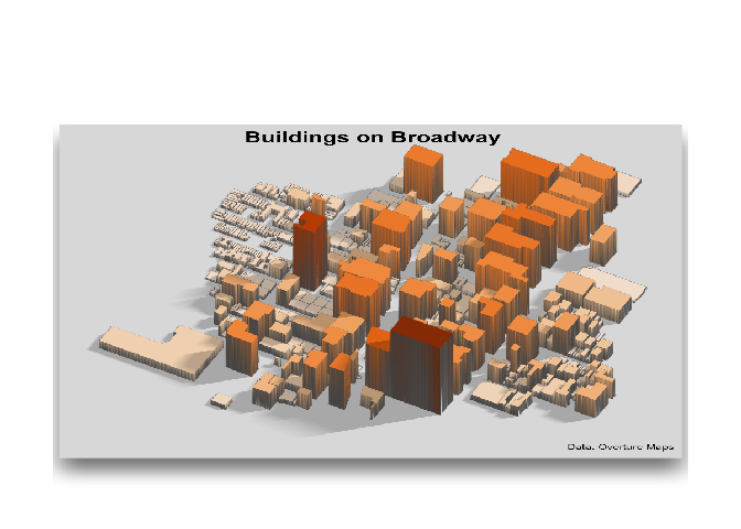
record_overture()mapgl)